Analysis Control Data

Individual header descriptions have been moved to the new manual. Only overviews and data definition examples are provided here.

Outline of Analysis Control Data

In FrontISTR, an analysis control data file is input to acquire the computing control data, solver control data and post process (visualization) control data as shown in the following figure, in order to implement the analytical calculations.

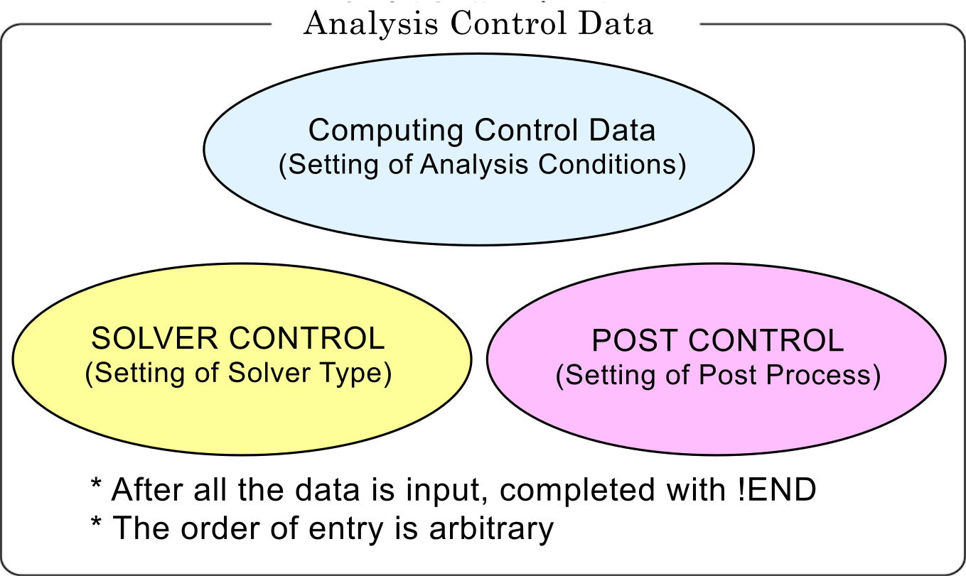
The features of the analysis control data file are as follows.

This is an ASCII format file based on a free format.
This file consists of a header which starts with "!" and the data following this.
The order of description of the header is basically free.
A "," is used as a punctuation mark of the data.
The inside of the file is briefly divided into three zones.
"!END" is input at the end of the file for completion.

Example of Analysis Control Data

#############################################################
##### (1) Computing control data portion ####################
#############################################################
### Control File for HEAT solver
!SOLUTION,TYPE=HEAT
!FIXTEMP
 XMIN, 0.0
 XMAX, 500.0

#############################################################
##### (2) Solver control data portion #######################
#############################################################
### Solver Control
!SOLVER,METHOD=1,PRECOND=1,ITERLOG=NO,TIMELOG=NO
100, 1
1.0e-8,1.0,0.0

#############################################################
##### (3) Post control (visualization) data portion #########
#############################################################
### Post Control
!WRITE,RESULT
!WRITE,VISUAL
!VISUAL, method=PSR
!surface_num = 1
!surface 1
!surface_style = 1
!display_method 1
!color_comp_name = TEMPERATURE
!color_subcomp = 1
!output_type = BMP
!x_resolution = 500
!y_resolution = 500
!num_of_lights = 1
!position_of_lights =
-20.0, 5.8, 80.0
!viewpoint = -20.0 10.0 8.0
!up_direction = 0.0 0.0 1.0
!ambient_coef= 0.3
!diffuse_coef= 0.7
!specular_coef= 0.5
!color_mapping_style= 1
!!interval_mapping= -0.01, 0.02
!color_mapping_bar_on = 1
!scale_marking_on = 1
!num_of_scale = 5
!font_size = 1.5
!font_color = 1.0 1.0 1.0
!END

Input Rules

The analysis control data consists of a header line, data line and a comment line.

One header is always included in the header line.

Header: The header specifies the meaning of the data and the data block in the analysis control data. When the head of the term starts with a "!", it is considered to be a header.
Header Line: The header and the parameter accompanying this are described in this line.; The header line must start with a header. When a parameter is required, a "," must be used to continue after that. When the parameter takes on a value, use an "=" after the parameter and describe the value after that.; The header line can not be described in more than two lines.
Data Line: The data line starts after the header line, and the necessary data is described.; The data lines may be in multiple lines; however, this is determined according to the rules of the data description defined by each header.; There are cases where data lines are not required.
Punctuation: A comma "," is used as a punctuation of the data.
Handling of Blanks: Blanks are disregarded.
Name: Regarding the characters which can be used for the name, there is the underscore "_", hyphen "-", and alphanumeric characters "a - z, A - Z, 0 - 9"; however, the first letter of the name must start with "_", or an alphabetic character "a - z, A - Z". There is no distinction between uppercase and lowercase letters, and all letters are internally handled as uppercase letters.; The maximum length of the name is 63 characters.
File Name: Regarding the characters which can be used for the file name, there are the underscore "_", hyphen "-", period ".", slash "/", and the alphanumeric characters "a - z, A - Z, 0 - 9".; As long as there is no specific description, a path can be included in the file name. Both the relative path and the absolute path can be specified.; The maximum length of the file name is 1,023 characters.
Floating Point Data: Exponents are optional. An "E" or "e" character must be added before the exponent. The selection of "E" or "e" is optional.
!!, #, Comment Line: Lines starting with "!!" or "#" are considered to be comment lines, and are disregarded. A comment line can be inserted in any position in the file, and there are no restrictions on the number of lines.
!END: End of mesh data; When this header is displayed, the reading of the mesh data is completed.

Analysis Control Data

Header List of Computing Control Data

In FrontISTR, the following items can be mentioned as the boundary conditions which can be used for the computing control data.

Distributed load conditions (body force, pressure loading, gravity, centrifugal force)
Concentrated load conditions
Heat load
Single point restriction conditions (SPC conditions)
Spring boundary conditions
Contact
Concentrated heat flux
Distributed heat flux
Convective heat transfer boundary
Radiant heat transfer boundary
Specified temperature boundary

The same as the mesh data, the !HEADER format is used as the definition method of the above boundary conditions.

The header list of the common control data is shown in the following Table 7.3.1, and the header list for each analysis type is shown in Table 7.3.2.

Table 7.3.1: Control Data Common to All Analysis

Header	Meaning	Remarks	Description No.
`!VERSION`	Solver version number		1-1
`!SOLUTION`	Specification of analysis type	Mandatory	1-2
`!WRITE,VISUAL`	Specification of visualization output		1-3
`!WRITE,RESULT`	Specification of results output		1-4
`!WRITE,LOG`	Specification of results output		1-5
`!OUTPUT_VIS`	Control of visualization output items		1-6
`!OUTPUT_RES`	Control of results output items		1-7
`!RESTART`	Control of restarting		1-8
`!ECHO`	Echo output		1-9
`!ORIENTATION`	Definition of local coordinate system		1-10
`!SECTION`	Definition of local coordinate system the sction correspondent to		1-11
`!INITIAL_CONDITION`	Definition of initial condition		1-12
`!END`	Ending specification of control data		1-13

Table 7.3.2: Control Data for Static Analysis

Header	Meaning	Description No.
`!STATIC`	Static analysis control	2-1
`!MATERIAL`	Material name	2-2
`!ELASTIC`	Elastic material physical properties	2-2-1
`!PLASTIC`	Plastic material physical properties	2-2-2
`!HYPERELASTIC`	Hyperelastic material physical properties	2-2-3
`!VISCOELASTIC`	Viscoelastic material physical properties	2-2-4
`!CREEP`	Creep material physical properties	2-2-5
`!DENSITY`	Mass density	2-2-6
`!EXPANSION_COEFF`	Coefficient of linear expansion	2-2-7
`!TRS`	Tempearture dependent behaviour of viscoelastic material	2-2-8
`!FLUID`	Flow Condition	2-2-9
`!USER_MATERIAL`	User defined material	2-2-10
`!BOUNDARY`	Displacement boundary conditions	2-3
`!SPRING`	Spring boundary conditions	2-3-1
`!CLOAD`	Concentrated load	2-4
`!DLOAD`	Distributed load	2-5
`!ULOAD`	User defined external load	2-6
`!CONTACT_ALGO`	Contact analytic algorithm	2-7
`!CONTACT`	Contact	2-8
`!TEMPERATURE`	Nodal temperature in thermal stress analysis	2-9
`!REFTEMP`	Reference temperature in thermal stress analysis	2-10
`!STEP`	Analysis step control	2-11
`!AUTOINC_PARAM`	Auto increment control	2-12
`!TIME_POINTS`	Output time point control	2-13
`!CONTACT_PARAM`	Contact scan control	2-14

Table 7.3.3: Control Data for Eigenvalue Analysis

Header	Meaning	Remarks	Description No.
`!EIGEN`	Eigenvalue analysis control	Mandatory in eigenvalue analysis	3-1

Table 7.3.4: Control Data for Heat Conduction Analysis

Header	Meaning	Remarks	Description No.
`!HEAT`	Heat conduction analysis control	Mandatory in heat conduction analysis	4-1
`!FIXTEMP`	Nodal temperature		4-2
`!CFLUX`	Concentrated heat flux given to node		4-3
`!DFLUX`	Distributed heat flux / internal heat generation given to element surface		4-4
`!SFLUX`	Distributed heat flux by surface group		4-5
`!FILM`	Heat transfer coefficient given to boundary plain		4-6
`!SFILM`	Heat transfer coefficient by surface group		4-7
`!RADIATE`	Radiation factor given to boundary plane		4-8
`!SRADIATE`	Radiation factor by surface group		4-9
`!WELD_LINE`	Weld line		4-10

Table 7.3.5: Control Data for Dynamic Analysis

Header	Meaning	Remarks	Description No.
`!DYNAMIC`	Dynamic analysis control	Mandatory in dynamic analysis	5-1
`!VELOCITY`	Velocity boundary conditions		5-2
`!ACCELERATION`	Acceleration boundary conditions		5-3
`!COUPLE`	Coupled surface definition Required in coupled analysis		5-4
`!EIGENREAD`	Specification of eigenvalues and eigenvectors	Mandatory in frequency response analysis	5-5
`!FLOAD`	Definition of concentrated load for frequency response analysis		5-6

In each header, there are data items which comply with the parameter and each header.

Each of the above headers is described in the following with examples of data creation for each analysis type. The description number in the above Table is the number indicated on the right end of the example of the data creation.

(1) Control data common to all analyses

Example of Analysis Control Data

### Control File for FISTR
!VERSION                                        1-1
  5
!SOLUTION, TYPE=STATIC                          1-2
!WRITE, VISUAL                                  1-3
!WRITE, RESULT                                  1-4
!ECHO                                           1-9
!BOUNDARY                                       2-3
  FIX, 1, 3, 0.0
!CLOAD                                          2-4
  CL1, 3, -1.0
!END                                            1-12

Description of Header

1-1 `!VERSION`

Refer to the solver version.

1-2 `!SOLUTION, TYPE=STATIC`

TYPE=analysis type

1-3 `!WRITE, VISUAL`

Output of data by visualizer via memory

Outputs the file just by entering

1-4 `!WRITE, RESULT`

Output of analysis results file

Outputs the file just by entering

1-6 `!ECHO`

Output of node data, element data and material data to log file

Outputs to the file just by entering

1-8 `!END`

Indicates the end of control data

(2) Static analysis control data

Example of Static Analysis Control data

### Control File for FISTR
!SOLUTION, TYPE=STATIC                          1-2
!WRITE, VISUAL                                  1-3
!WRITE, RESULT                                  1-4
!ECHO                                           1-9
!MATERIAL, NAME=M1                              2-2
!ELASTIC, TYPE=ISOTROPIC                        2-2-1
  210000.0, 0.3
!BOUNDARY                                       2-3
  FIX, 1, 3, 0.0
!SPRING 2-3-1
  200, 1, 0.03
!CLOAD 2-4
  CL1, 3, -1.0
!DLOAD 2-5
  1, P1, 1.0
!TEMPERATURE                                    2-9
  1, 10.0
!REFTEMP                                        2-10
!STEP, CONVERG=1.E-5, MAXITER=30                2-11
!END                                            1-12

Description of Header

Red figures are the values indicated in the example.
Alphabetic characters in the 2nd line of the table express the parameter name.

2-1 `!STATIC`

Setting of static analysis method

2-2 `!MATERIAL`

Definition of material physical properties

NAME = name of material physical properties

2-2-1 `!ELASTIC, TYPE=ISOTROPIC`

Definition of elastic substance

TYPE = elastic type

Young's Modulus	Poisson's Ratio
YOUNG_MODULUS	POISSON_RATIO
210000.0	0.3

2-3 `!BOUNDARY`

Definition of displacement boundary conditions

Node ID or Node Group Name	Start No. of Restricted Degree of Freedom	End No. of Restricted Degree of Freedom	Restricted Value
NODE_ID	DOF_idS	DOF_idE	Value
FIX,	1,	3,	0.0

2-3-1 `!SPRING`

Definition of spring boundary conditions

Node ID or Node Group Name	Restricted Degree of Freedom	Spring Constant
NODE_ID	DOF_id	Value
200,	1,	0.03

2-4 `!CLOAD`

Definition of concentrated load

Node ID or Node Group Name	Degree of Freedom No.	Load Value
NODE_ID	DOF_id	Value
CL1,	3,	-1.0

2-5 `!DLOAD`

Definition of distributed load

Element ID or Element Group Name	Load Type No.	Load Parameter
ELEMENT_ID	LOAD_type	param
1,	P1,	1.0

2-9 `!TEMPERATURE`

Specification of nodal temperature used for thermal stress analysis

Node ID or Node Group Name	Temperature
NODE_ID	Temp_Value
1,	10

2-10 `!REFTEMP`

Definition of reference temperature in thermal stress analysis

2-11 `!STEP`

Control of nonlinear static analysis (Omissible in the case of linear analysis)

Convergence Value Judgment Threshold	No. of Sub Steps (When AMP exists, AMP has priority)	Max No. of Iterative Calculations	Time Function Name (Specified in `!AMPLITUDE`)
CONVERG	SUBSTEPS	MAXITER	AMP
1.0E-05	10	30

(3) Eigenvalue analysis control data

Example of Eigenvalue Analysis Control Data

### Control File for FISTR
!SOLUTION, TYPE=EIGEN                           1-2
!WRITE, VISUAL                                  1-3
!WRITE, RESULT                                  1-4
!ECHO                                           1-9
!EIGEN                                          3-1
  3, 1.0E-8, 60
!BOUNDARY                                       2-3
 FIX, 1, 2, 0.0
!END

Description of Header

Red figures are the values indicated in the example.

3-1 `!EIGEN`

Parameter settings of eigenvalue analysis

No. of Eigenvalue	Allowance	Max No. of Iterations
NSET	LCZTOL	LCZMAX
3,	1.0E-8,	60

2-3 `!BOUNDARY` (Same items an in Static Analysis)

Definition of displacement boundary conditions

Node ID or Node Group Name	Start No. of Restricted Degree of Freedom	End No. of Restricted Degree of Freedom	Restricted Value
NODE_ID	DOF_idS	DOF_idE	Value
FIX,	1,	3,	0.0

(4) Heat conduction analysis control data

Example of Heat Conduction Analysis Control Data

### Control File for FISTR
!SOLUTION, TYPE=HEAT                            1-2
!WRITE, VISUAL                                  1-3
!WRITE, RESULT                                  1-4
!ECHO                                           1-9
!HEAT                                           4-1
!FIXTEMP                                        4-2
  XMIN, 0.0
  XMAX, 500.0
!CFLUX                                          4-3
  ALL, 1.0E-3
!DFLUX                                          4-4
  ALL, S1, 1.0
!SFLUX                                          4-5
  SURF, 1.0
!FILM                                           4-6
  FSURF, F1, 1.0, 800
!SFILM                                          4-7
  SFSURF, 1.0, 800.0
!RADIATE                                        4-8
  RSURF, R1, 1.0E-9, 800.0
!SRADIATE                                       4-9
  RSURF, R1, 1.0E-9, 800.0
!END                                            1-12

Description of Header

Red figures are the values indicated in the example.

4-1 `!HEAT`

Definition of control data for calculation

!HEAT
  (No data)                         ----- Steady calculation
!HEAT
  0.0                               ----- Steady calculation
!HEAT
  10.0, 3600.0                      ----- Fixed time increment unsteady calculation
!HEAT
  10.0, 3600.0, 1.0                 ----- Automatic time increment unsteady calculation
!HEAT
  10.0, 3600.0, 1.0, 20.0           ----- Automatic time increment unsteady calculation

4-2 `!FIXTEMP`

Node group name, or node ID and fixed temperature

4-3 `!CFLUX`

Definition of concentrated heat flux given to node

Node Group Name or Node ID	Heat Flux Value
NODE_GRP_NAME	Value
ALL,	1.0E-3

4-4 `!DFLUX`

Definition of distributed heat flux and internal heat generation given to surface of element

Element Group Name or Element ID	Load Type No.	Heat Flux Value
ALL,	S1,	1.0

Load Parameter

Load Type No.	Applied Surface	Parameter
BF	Element Overall	Calorific value
S1	Surface No. 1	Heat flux value
S2	Surface No. 2	Heat flux value
S3	Surface No. 3	Heat flux value
S4	Surface No. 4	Heat flux value
S5	Surface No. 5	Heat flux value
S6	Surface No. 6	Heat flux value
S0	Shell surface	Heat flux value

4-5 `!SFLUX`

Definition of distributed heat flux by surface group

Surface Group Name	Heat Flux Value
SURFACE_GRP_NAME	Value
SURF,	1.0

4-6 `!FILM`

Definition of heat transfer coefficient given to boundary plane

Element Group Name or Element ID	Load Type No.	Heat Transfer Coefficient	Ambient Temperature
ELEMENT_GRP_NAME	LOAD_type	Value	Sink
FSURF,	F1,	1.0,	800.0

Load Parameter

Load Type No.	Applied Surface	Parameter
F1	Surface No. 1	Heat transfer coefficient and ambient temperature
F2	Surface No. 2	Heat transfer coefficient and ambient temperature
F3	Surface No. 3	Heat transfer coefficient and ambient temperature
F4	Surface No. 4	Heat transfer coefficient and ambient temperature
F5	Surface No. 5	Heat transfer coefficient and ambient temperature
F6	Surface No. 6	Heat transfer coefficient and ambient temperature
F0	Shell surface	Heat transfer coefficient and ambient temperature

4-7 `!SFILM`

Definition of heat transfer coefficient by surface group

Surface Group Name	Heat Transfer Rate	Ambient Temperature
SURFACE_GRP_NAME	Value	Sink
SFSURF,	1.0,	800.0

4-8 `!RADIATE`

Definition of radiation factor given to boundary plane

Element Group Name or Element ID	Load Type No.	Radiation Factor	Ambient Temperature
ELEMENT_GRP_NAME	LOAD_type	Value	Sink
RSURF,	R1,	1.0E-9,	800.0

Load Parameter

Load Type No.	Applied Surface	Parameter
R1	Surface No. 1	Radiation factor and ambient temperature
R2	Surface No. 2	Radiation factor and ambient temperature
R3	Surface No. 3	Radiation factor and ambient temperature
R4	Surface No. 4	Radiation factor and ambient temperature
R5	Surface No. 5	Radiation factor and ambient temperature
R6	Surface No. 6	Radiation factor and ambient temperature
R0	Shell surface	Radiation factor and ambient temperature

4-9 `!SRADIATE`

Definition of radiation factor by surface group

Surface Group Name	Radiation Factor	Ambient Temperature
SURFACE_GRP_NAME	Value	Sink
SRSURF,	1.0E-9,	800.0

(5) Dynamic analysis control data

Example of Dynamic Analysis Control Data

### Control File for FISTR
!SOLUTION, TYPE=DYNAMIC                         1-2
!DYNAMIC, TYPE=NONLINEAR                        5-1
  1 , 1
  0.0, 1.0, 500, 1.0000e-5
  0.5, 0.25
  1, 1, 0.0, 0.0
  100, 5, 1
  0, 0, 0, 0, 0, 0
!BOUNDARY, AMP=AMP1                             2-3
  FIX, 1, 3, 0.0
!CLOAD, AMP=AMP1                                2-4
  CL1, 3, -1.0
!COUPLE, TYPE=1                                 5-4
  SCOUPLE
!STEP, CONVERG=1.E-6, ITMAX=20                  2-11
!END                                            1-12

Description Header

Red figures are the values indicated in the example.
Alphabetic characters in the 2nd line of the table express the parameter name.

5-1 `!DYNAMIC`

Controlling the linear dynamic analysis

Solution of Equation of Motion	Analysis Types
idx_eqa	idx_resp
11	1

Analysis Start Time	Analysis End Time	Overall No. of STEPS	Time Increment
t_start	t_end	n_step	t_delta
0.0	1.0	500	1.0000e-5

Parameter $\gamma$ of Newmark- $\beta$ Method	Parameter $\beta$ of Newmark- $\beta$ Method
gamma	beta
0.5	0.25

Type of Mass Matrix	Type of Damping	Parameter $R_m$ of Rayleigh Damping	Parameter of $R_k$ of Rayleigh Damping
idx_mass	idx_dmp	ray_m	ray_k
1	1	0.0	0.0

Resules Output Interval	Monitoring Node ID or Node Group Name	Results Output Interval of Displacement Monitoring
nout	node_monit_1	nout_monit
100	55	nout_monit

Output Control Displacement	Output Control Velocity	Output Control Acceleration	Output Control Reaction Force	Output Control Strain	Output Control Stress
iout_list(1)	iout_list(2)	iout_list(3)	iout_list(4)	iout_list(5)	iout_list(6)
0	0	0	0	0	0

2-3 `!BOUNDARY` (Same items as in Static Analysis)

Definition of displacement boundary conditions

Node ID or Node Group Name	Start No. of Restricted Degree of Freedom	End No. of Restricted Degree of Freedom	Restricted Value
NODE_ID	DOF_idS	DOF_idE	Value
FIX,	1,	3,	0.0

2-4 `!CLOAD` (Same items as in Static Analysis)

Definition of concentrated load

Node ID or Node Group Name	Degree of Freedom No.	Load Value
CL1,	3,	-1.0

5-4 `!COUPLE, TYPE=1`

Definition of coupled surface

Coupling Surface Group Name
SCOUPLE

2-11 `!STEP, CONVERG=1.E-10, ITMAX=20`

Control of nonlinear static analysis

(Omissible in the case of linear analysis, and unnecessary for explicit method)

Convergence Value Judgment Threshold (Default: 1.0E-06)	No. of Sub Steps (When AMP exists, AMP has priority)	Max No. of Iterative Calculations
CONVERG	SUBSTEPS	ITMAX
1.0E-10		20

(6) Dynamic analysis (Frequency Response Analysis) Control Data

Example of Dynamic analysis (Frequency Response Analysis)

!SOLUTION, TYPE=DYNAMIC                         1-2
!DYNAMIC                                        5-1
  11 , 2
  14000, 16000, 20, 15000.0
  0.0, 6.6e-5
  1, 1, 0.0, 7.2E-7
  10, 2, 1
  1, 1, 1, 1, 1, 1
!EIGENREAD                                      5-5
  eigen0.log
  1, 5
!FLOAD, LOAD CASE=2                             5-6
  _PickedSet5, 2, 1.0
!FLOAD, LOAD CASE=2
  _PickedSet6, 2, 1.0

Description of Header

Red figures are the values indicated in the example.
Alphabetic characters in the 2nd line of the table express the parameter name.

5-1 `!DYNAMIC`

Controlling the frequency response analysis

Solution of Equation of Motion	Analysis Types
idx_eqa	idx_resp
11	2

Minimum Frequency	Maximum Frequency	Number of divisions for the frequency range	Frequency to obtain displacement
f_start	f_end	n_freq	f_disp
14000	16000	20	15000.0

Analysis Start Time	Analysis End Time
0.0	6.6e-5

Type of Mass Matrix	Type of Damping	Parameter $R_m$ of Rayleigh Damping	Parameter $R_k$ of Rayleigh Damping
idx_mass	idx_dmp	ray_m	ray_k
1	1	0.0	7.2E-7

Results Output Interval in Time Domain	Visualization Type (1-Mode shapes, 2-Time history result at f_disp)	Monitoring Node ID in Frequency Domain
nout	vistype	nodeout
10	2	1

Output Control Displacement	Output Control Velocity	Output Control Acceleration	Output Control ignored	Output Control ignored	Output Control ignored
iout_list(1)	iout_list(2)	iout_list(3)	iout_list(4)	iout_list(5)	iout_list(6)
1	1	1	1	1	1

5-5 `!EIGENREAD`

Controlling the input file for frequency response analysis

The name of eigenvalue analysis log
eigenlog_filename
eigen0.log

lowest mode to be used in frequency response analysis	highest mode to be used frequency response analysis
start_mode	end_mode
1	5

5-6 `!FLOAD`

Defining external forces applied in frequency response analysis

Node ID, Node Group Name or Surface Group Name	Degree of Freedom No.	Load Value
_PickedSet5	2	1.0

Solver Control Data

Example of Solver Control Data

### SOLVER CONTROL
!SOLVER, METHOD=CG, PRECOND=1, ITERLOG=YES, TIMELOG=YES        6-1
  10000, 1                                                     6-2
  1.0e-8, 1.0, 0.0

Description of Header

Red figures are the values indicated in the example.

6-1 `!SOLVER`

METHOD    = method
           (CG, BiCGSTAB, GMRES, GPBiCG, etc.)
TIMELOG   = whether solver computation time is output
MPCMETHOD = method for multipoint constraints
            (1: Penalty method,
             2: MPC-CG method (Deprecated),
             3: Explicit master-slave elimination)
DUMPTYPE  = type of matrix dumping
DUMPEXIT  = whether program exits right after dumping matrix

The following parameters will be disregarded when a direct solver is selected in the method.

PRECOND   = preconditioner
ITERLOG   = whether solver convergence history is output
SCALING   = whether matrix is scaled so that each diagonal element becomes 1
USEJAD    = whether matrix ordering optimized for vector processors is performed
ESTCOND   = frequency for estimating condition number
            (Estimation performed at every specified number of iterations and
             at the last iteration.  No estimation when 0 is specified.)

6-2

No. of Iterations	Iteration Count of Preconditioning	No. of Krylov Subspaces	No. of Colors for Multi-Color ordering	No. of Recycling Set-Up Info for Preconditioning
NITER	iterPREMAX	NREST	NCOLOR_IN	RECYCLEPRE
10000	1

6-3

Truncation Error	Scale Factor for Diagonal Elements when computing Preconditioning Matrix	Not Used
1.0e-8,	1.0,	0.0

Post Process (Visualization) Control Data

An example of the post process (visualization) control data and the contents are shown in the following.

Example of Visualization Control Data

Each description number (P1-0, P1-1, etc.) is linked to the number of the detailed descriptions in the following.

P1-○ expresses the common data, and P2-○ expresses the parameter for the purpose of the rendering.
In addition, the rendering will become valid only when the output_type=BMP.
When the surface_style is !surface_style = 2 (isosurface) !surface_style = 3 (user specified curved surface), a separate setting is required. The data is indicated collectively after the common data.
(P3-○ is a description of the isosurface in !surface_style = 2. P4-○ is a description of the user specified curved surface in !surface_style = 3.)
The items indicated with two ! like "!!", will be recognized as a comment and will not affect the analysis.

### Post Control                                Description No.
!VISUAL, method=PSR                             P1-0
!surface_num = 1                                P1-1
!surface 1                                      P1-2
!surface_style = 1                              P1-3
!display_method = 1                             P1-4
!color_comp_name = STRESS                       P1-5
!colorsubcomp_name                              P1-6
!color_comp 7                                   P1-7
!!color_subcomp = 1                             P1-8
!iso_number                                     P1-9
!specified_color                                P1-10
!deform_display_on = 1                          P1-11
!deform_comp_name                               P1-12
!deform_comp                                    P1-13
!deform_scale = 9.9e-1                          P1-14
!initial_style = 1                              P1-15
!deform_style = 3                               P1-16
!initial_line_color                             P1-17
!deform_line_color                              P1-18
!output_type = BMP                              P1-19
!x_resolution = 500                             P2-1
!y_resolution = 500                             P2-2
!num_of_lights = 1                              P2-3
!position_of_lights = -20.0, 5.8, 80.0          P2-4
!viewpoint = -20.0 -10.0 5.0                    P2-5
!look_at_point                                  P2-6
!up_direction = 0.0 0.0 1.0                     P2-7
!ambient_coef= 0.3                              P2-8
!diffuse_coef= 0.7                              P2-9
!specular_coef= 0.5                             P2-10
!color_mapping_style= 1                         P2-11
!!interval_mapping_num                          P2-12
!interval_mapping= -0.01, 0.02                  P2-13
!rotate_style = 2                               P2-14
!rotate_num_of_frames                           P2-15
!color_mapping_bar_on = 1                       P2-16
!scale_marking_on = 1                           P2-17
!num_of_scale = 5                               P2-18
!font_size = 1.5                                P2-19
!font_color = 1.0 1.0 1.0                       P2-20
!background_color                               P2-21
!isoline_color                                  P2-22
!boundary_line_on                               P2-23
!color_system_type                              P2-24
!fixed_range_on = 1                             P2-25
!range_value = -1.E-2, 1.E-2                    P2-26

Common Data List<P1-1 - P1-19>

No.	Keywords	Types	Contents
P1-0	`!VISUAL`		Specification of the visualization method
P1-1	`surface_num`		No. of surfaces in one surface rendering
P1-2	`surface`		Setting of the contents of surface
P1-3	`surface_style`	integer	Specification of the surface type (Default: 1) 1: Boundary surface 2: Isosurface 3: Curved surface defined by user based on the equation
P1-4	`display_method`	integer	Display method (Default: 1) 1. Color code display 2. Boundary line display 3. Color code and boundary line display 4. Display of 1 specified color 5. Isopleth line display by classification of color
P1-5	`color_comp_name`	character(100)	Compatible with parameter name and colormap (Default: 1st parameter name)
P1-6	`color_subcomp_name`	character(4)	When the parameter is a vector, specifies the component to be displayed. (Default: x) norm: Norm of the vector x: x component y: y component z: z component
P1-7	`color_comp`	integer	Provides an ID number to the parameter name (Default: 0)
P1-8	`color_subcomp`	integer	When the degree of freedom of the parameter is 1 or more, specifies the degree of freedom number to be displayed. 0: Norm (Default: 1)
P1-9	`iso_number`	integer	Specifies the number of isopleth lines. (Default:5)
P1-10	`specified_color`	real	Specified the color when the `display_method = 4` 0.0 < specified_color < 1.0
P1-11	`!deform_display_on`	integer	Specifies the existence of deformation. 1: On, 0: Off (Default: 0)
P1-12	`!deform_comp_name`	character(100)	Specifies the attribution to be adopted when specifying deformation. (Default: Parameter called DISPLCEMENT)
P1-13	`!deform_ comp`	integer	ID number of the parameter when specifying deformation. (Default: 0)
P1-14	`!deform_scale`	real	Specifies the displacement scale when displaying deformation. Default:Auto `standard_scale` = 0.1 * sqrt(`x_range`² + `y_range`² + `z_range`²) / `max_deform` `user_defined`: `real_scale` = `standard_scale` * `deform_scale`
P1-15	`!initial_style`	integer	Specifies the type of deformation display.(Default: 1) 0: Not specified 1: Solid line mesh(Displayed in blue if not specified) 2: Gray filled pattern 3: Shading (Let the physical attributions respond to the color) 4: Dotted line mesh (Displayed in blue if not specified)
P1-16	`!deform_style`	integer	Specifies the shape display style after the initial deformation.(Default: 4) 0: Not specified 1: Solid line mesh (Displayed in blue if not specified) 2: Gray filled pattern 3: Shading (Let the physical attributions respond to the color) 4: Dotted line mesh (Displayed in blue if not specified)
P1-17	`!initial_line_color`	real (3)	Specifies the color when displaying the initial mesh. This includes both the solid lines and dotted lines. (Default: Blue(0.0, 0.0, 1.0))
P1-18	`!deform_line_color`	real (3)	Specifies the color when displaying the deformed mesh. This includes both the solid lines and dotted lines. (Yellow(1.0, 1.0, 0.0))
P1-19	`output_type`	character(3)	Specifies the type of output file. (Default: AVS) `AVS`: UCD Data for AVS(only on object surface) `BMP`: Image data (BMP format) `COMPLETE_AVS`: UCD data for AVS `COMPLETE_REORDER_AVS`: Rearranges the node and element ID `SEPARATE_COMPLETE_AVS`: For each decomposed domain `COMPLETE_MICROAVS`: Outputs the physical value scalar `FSTR_FEMAP_NEUTRAL`: Neutral file for FEMAP

Rendering Data List <P2-1 - P2-26>

(Valid only when the output_type=BMP)

	Keywords	Types	Contents
P2-1	`x_resolution`	integer	Specifies the width of final figure. (Default: 512)
P2-2	`y_resolution`	integer	Specifies the height of final figure. (Default: 512)
P2-3	`num_of_lights`	integer	Specifies the number of lights. (Default: 1)
P2-4	`position_of_lights`	real(:)	Specifies the position of the lights by coordinates.(Default: Directly above front) Specification method `!position_of_lights= x, y, z, x, y, z,...` Ex) `!position_of_lights=100.0, 200.0, 0.0`
P2-5	`viewpoint`	real(3)	Specifies the viewpoint position by coordinates. (Default: x = (x_min + x_max)/2.0) y = y_min + 1.5 ( y_max - y_min) z = z_min + 1.5 ( z_max - z_min) )
P2-6	`look_at_point`	real(3)	Specifies the look at point position. (Default: Center of data)
P2-7	`up_direction`	real(3)	Defines the view frame at Viewpoint, `look_at_point` and `up_direction` (Default: 0.0, 0.0, 1.0)
P2-8	`ambient_coef`	real	Specifies the peripheral brightness. (Default: 0.3)
P2-9	`diffuse_coef`	real	Specifies the intensity of the diffused reflection light by coefficient. (Default: 0.7)
P2-10	`specular_coef`	real	Specifies the intensity of specular reflection by coefficient. (Default: 0.6)
P2-11	`color_mapping_style`	integer	Specifies the color mapping style. (Default: 1) 1: Complete linear mapping (Maps overall color in RGB linear) 2: Clip linear mapping (Maps from `mincolor` to `maxcolor` in the RGB color space) 3: Nonlinear color mapping (Patitions all domains into multiple sections, and performs linear mapping for each section) 4: Optimum auto adjustment (Performs a statistical process of the data distribution to determine the color mapping)
P2-12	`interval_mapping_num`	integer	Specifies the number of sections when the `color_mapping_style = 3`
P2-13	`interval_mapping`	real(:)	Specifies the section position and color number when the `color_mapping_style = 2` or `3`. if the `color_mapping_style=2`; `!interval_mapping=[minimum color], [maximum color]` If the `color_mapping_style=3`; `!interval_mapping=[section,compatible color value],... repeats number specified` Note: Must be describe in one line.
P2-14	`rotate_style`	integer	Specifies the rotating axis of animation. 1: Rotates at x-axis. 2: Rotates at y-axis. 3: Rotates at z axis. 4: Particularly, specifies the viewpoint to perform animation. (8 frames)
P2-15	`rotate_num_of_frames`	integer	Specifies the cycle of animation. (`rotate_style` = 1, 2, 3) (Default: 8)
P2-16	`color_mapping_bar_on`	integer	Specifies the existence of color mapping bar. 0: off; 1: on; Default: 0
P2-17	`scale_marking_on`	integer	Specifies whether to display the value on the color mapping bar. 0: off; 1: on; Default: 0
P2-18	`num_of_scale`	integer	Specifies the number of memories of the color bar. (Default: 3)
P2-19	`font_size`	real	Specifies the font size when displaying the value of the color mapping bar. Range: 1.0-4.0 (Default: 1.0)
P2-20	`font_color`	real(3)	Specifies the display color when displaying the value of the color mapping bar. (Default: 1.0, 1.0, 1.0 (White))
P2-21	`background_color`	real(3)	Specifies the background color. (Default: 0.0, 0.0, 0.0 (Black))
P2-22	`isoline_color`	real(3)	Specifies the color of the isopleth line. (Default: Same color as the value)
P2-23	`boundary_line_on`	integer	Specifies whether to display the zone of the data. 0: off; 1: on; Default: 0
P2-24	`color_system_type`	integer	Specifies the color mapping style. (Default: 1) 1: (Blue - Red)(in ascending order) 2: Rainbow mapping (Ascending order from red to purple) 3: (Black - White)(in ascending order)
P2-25	`fixed_range_on`	integer	Specifies whether to maintain the color mapping style for other time steps. 0: off; 1: on; (Default: 0)
P2-26	`range_value`	real(2)	Specifies the section.

Data List by Setting Values of `surface_style`

In the case of isosurface (`surface_style=2`)

	Keywords	Types	Contents
P3-1	`data_comp_name`	character(100)	Provides the name to the attribution of the isosurface.
P3-2	`data_subcomp_name`	character(4)	When the parameter is a vector, specifies the component to be displayed. (Default: x) norm: Norm of the vector x: x component y: y component z: z component
P3-3	`data_comp`	integer	Provides an ID number to the parameter name (Default: 0)
P3-4	`data_subcomp`	integer	When the degree of freedom of the parameter is 1 or more, specifies the degree of freedom number to be displayed. 0: Norm (Default: 1)
P3-5	`iso_value`	real	Specifies the value of the isosurface.

In the case of a curved surface (surface_sytle = 3) specified by the equation of the user

	Keywords	Types	Contents
P4-1	method	integer	Specifies the attribution of the curved surface. (Default: 5) 1: Spherical surface 2: Ellipse curved surface 3: Hyperboloid 4: Paraboloid 5: General quadric surface
P4-2	point	real(3)	Specifies the coordinates of the center when method = 1, 2, 3, or 4 (Default: 0.0, 0.0, 0.0)
P4-3	radius	real	Specifies the radius when method = 1 (Default: 1.0)
P4-4	length	real	Specifies the length of the diameter when method = 2, 3, or 4. Note: The length of one diameter in the case the ellipse curved surface is 1.0.
P4-5	coef	real	Specifies the coefficient of a quadric surface when method=5. coef[1]x² + coef[2]y² + coef[3]z² + coef[4]xy + coef[5]xz + coef[6]yz + coef[7]x + coef[8]y + coef[9]z + coef[10]=0 Ex: coef=0.0, 0.0, 0.0, 0.0, 0.0, 0.0, 0.0, 1.0, 0.0, -10.0 This means the plain surface of y=10.0

Analysis Control Data

Analysis Control Data

Outline of Analysis Control Data

Input Rules

Analysis Control Data

Header List of Computing Control Data

(1) Control data common to all analyses

Example of Analysis Control Data

Description of Header

1-1 !VERSION

1-2 !SOLUTION, TYPE=STATIC

1-3 !WRITE, VISUAL

1-4 !WRITE, RESULT

1-6 !ECHO

1-8 !END

(2) Static analysis control data

Example of Static Analysis Control data

Description of Header

2-1 !STATIC

2-2 !MATERIAL

2-2-1 !ELASTIC, TYPE=ISOTROPIC

2-3 !BOUNDARY

2-3-1 !SPRING

2-4 !CLOAD

2-5 !DLOAD

2-9 !TEMPERATURE

2-10 !REFTEMP

2-11 !STEP

(3) Eigenvalue analysis control data

Example of Eigenvalue Analysis Control Data

Description of Header

3-1 !EIGEN

2-3 !BOUNDARY (Same items an in Static Analysis)

(4) Heat conduction analysis control data

Example of Heat Conduction Analysis Control Data

Description of Header

4-1 !HEAT

4-2 !FIXTEMP

4-3 !CFLUX

4-4 !DFLUX

4-5 !SFLUX

4-6 !FILM

4-7 !SFILM

4-8 !RADIATE

4-9 !SRADIATE

(5) Dynamic analysis control data

Example of Dynamic Analysis Control Data

Description Header

5-1 !DYNAMIC

2-3 !BOUNDARY (Same items as in Static Analysis)

2-4 !CLOAD (Same items as in Static Analysis)

5-4 !COUPLE, TYPE=1

2-11 !STEP, CONVERG=1.E-10, ITMAX=20

(6) Dynamic analysis (Frequency Response Analysis) Control Data

Example of Dynamic analysis (Frequency Response Analysis)

Description of Header

5-1 !DYNAMIC

5-5 !EIGENREAD

5-6 !FLOAD

Solver Control Data

Example of Solver Control Data

Description of Header

6-1 !SOLVER

6-2

6-3

Post Process (Visualization) Control Data

Example of Visualization Control Data

Common Data List<P1-1 - P1-19>

Rendering Data List <P2-1 - P2-26>

Data List by Setting Values of surface_style

In the case of isosurface (surface_style=2)

In the case of a curved surface (surface_sytle = 3) specified by the equation of the user

1-1 `!VERSION`

1-2 `!SOLUTION, TYPE=STATIC`

1-3 `!WRITE, VISUAL`

1-4 `!WRITE, RESULT`

1-6 `!ECHO`

1-8 `!END`

2-1 `!STATIC`

2-2 `!MATERIAL`

2-2-1 `!ELASTIC, TYPE=ISOTROPIC`

2-3 `!BOUNDARY`

2-3-1 `!SPRING`

2-4 `!CLOAD`

2-5 `!DLOAD`

2-9 `!TEMPERATURE`

2-10 `!REFTEMP`

2-11 `!STEP`

3-1 `!EIGEN`

2-3 `!BOUNDARY` (Same items an in Static Analysis)

4-1 `!HEAT`

4-2 `!FIXTEMP`

4-3 `!CFLUX`

4-4 `!DFLUX`

4-5 `!SFLUX`

4-6 `!FILM`

4-7 `!SFILM`

4-8 `!RADIATE`

4-9 `!SRADIATE`

5-1 `!DYNAMIC`

2-3 `!BOUNDARY` (Same items as in Static Analysis)

2-4 `!CLOAD` (Same items as in Static Analysis)

5-4 `!COUPLE, TYPE=1`

2-11 `!STEP, CONVERG=1.E-10, ITMAX=20`

5-1 `!DYNAMIC`

5-5 `!EIGENREAD`

5-6 `!FLOAD`

6-1 `!SOLVER`

Data List by Setting Values of `surface_style`

In the case of isosurface (`surface_style=2`)