Example of Acutual Model for Elastic Static Analysis

Actual Model Examples for Elastic Static Analysis

Analysis Model

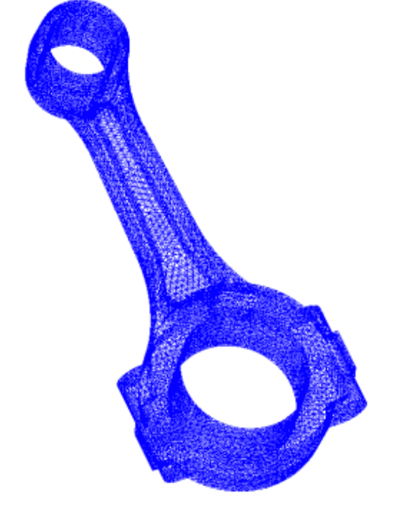
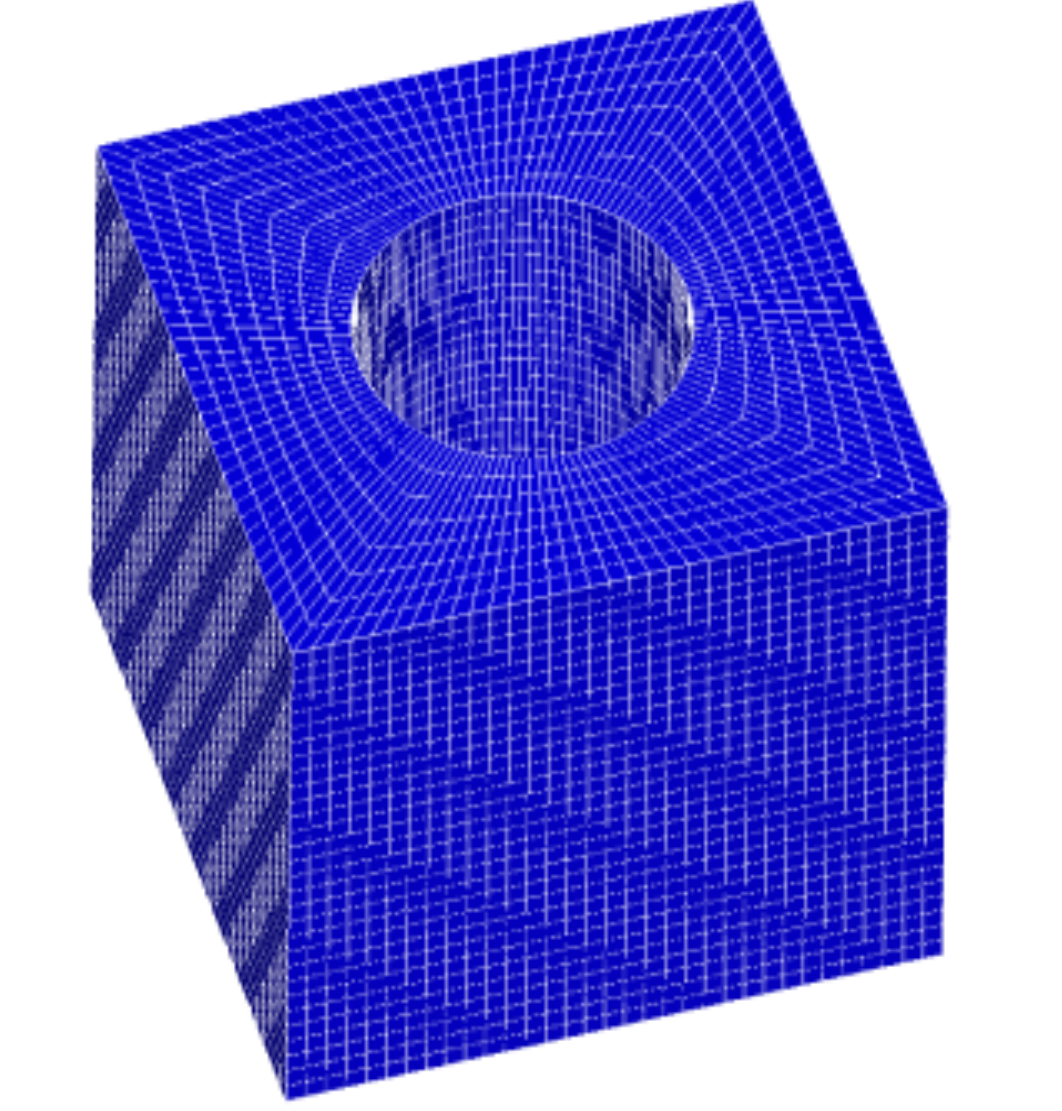
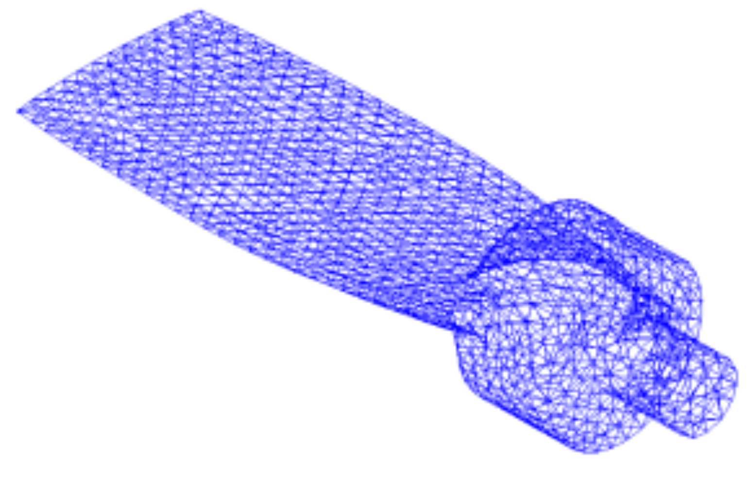
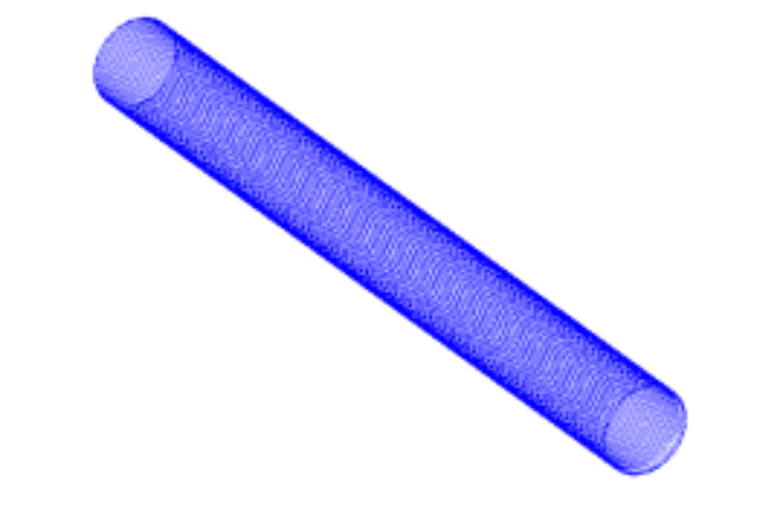
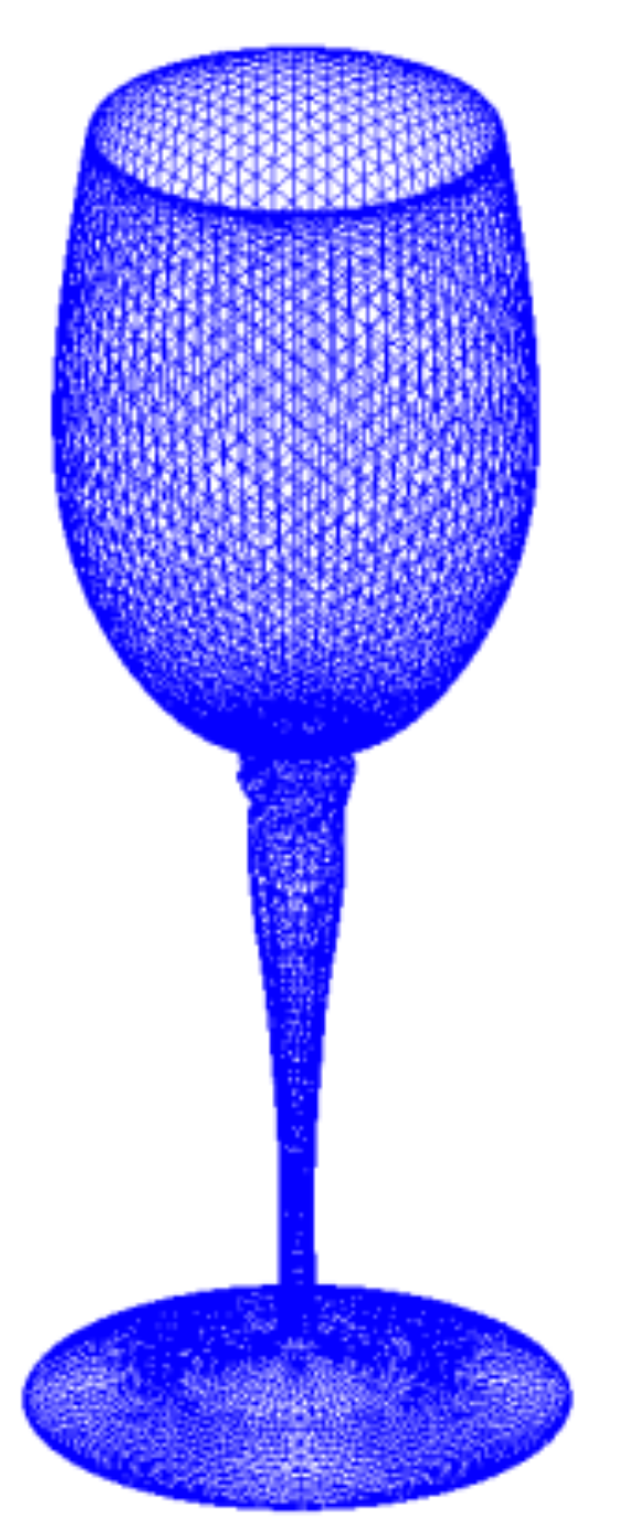
A list of actual model verification examples for elastic static analysis are presented in Table 9.2.1. The different shapes of the models are shown in Figs. 9.2.1–9.2.5 (some models are excluded). The examples of the element types 731 and 741 require a separate direct method solver.

Table 9.2.1: Actual model verification examples for elastic static analysis

Case name	Element type	Verification model	Number of nodes	Freedom freequency
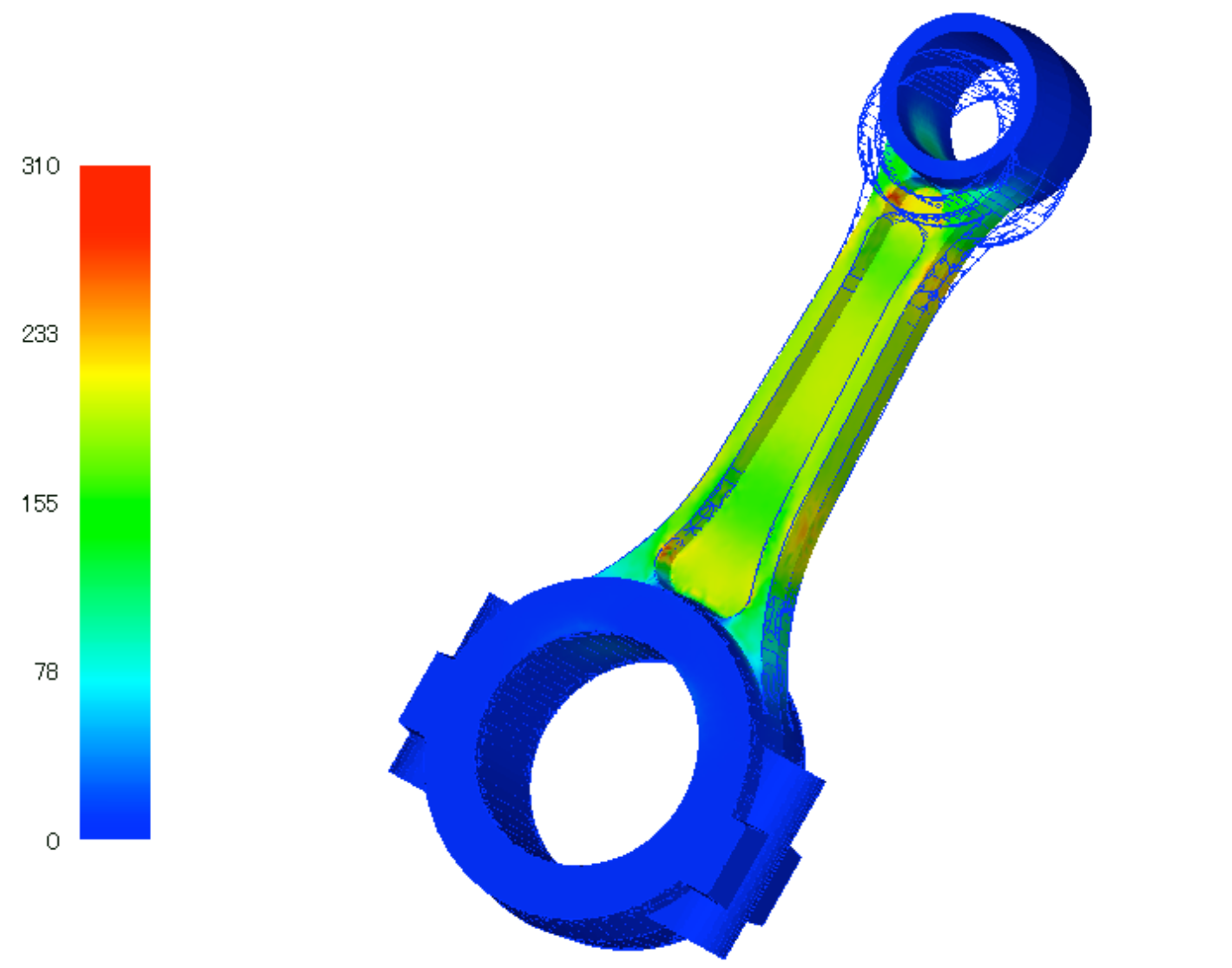
EX01A	342	Connecting rod (100,000 nodes)	94,074	282,222
EX01B	342	Connecting rod (330,000 nodes)	331,142	993,426
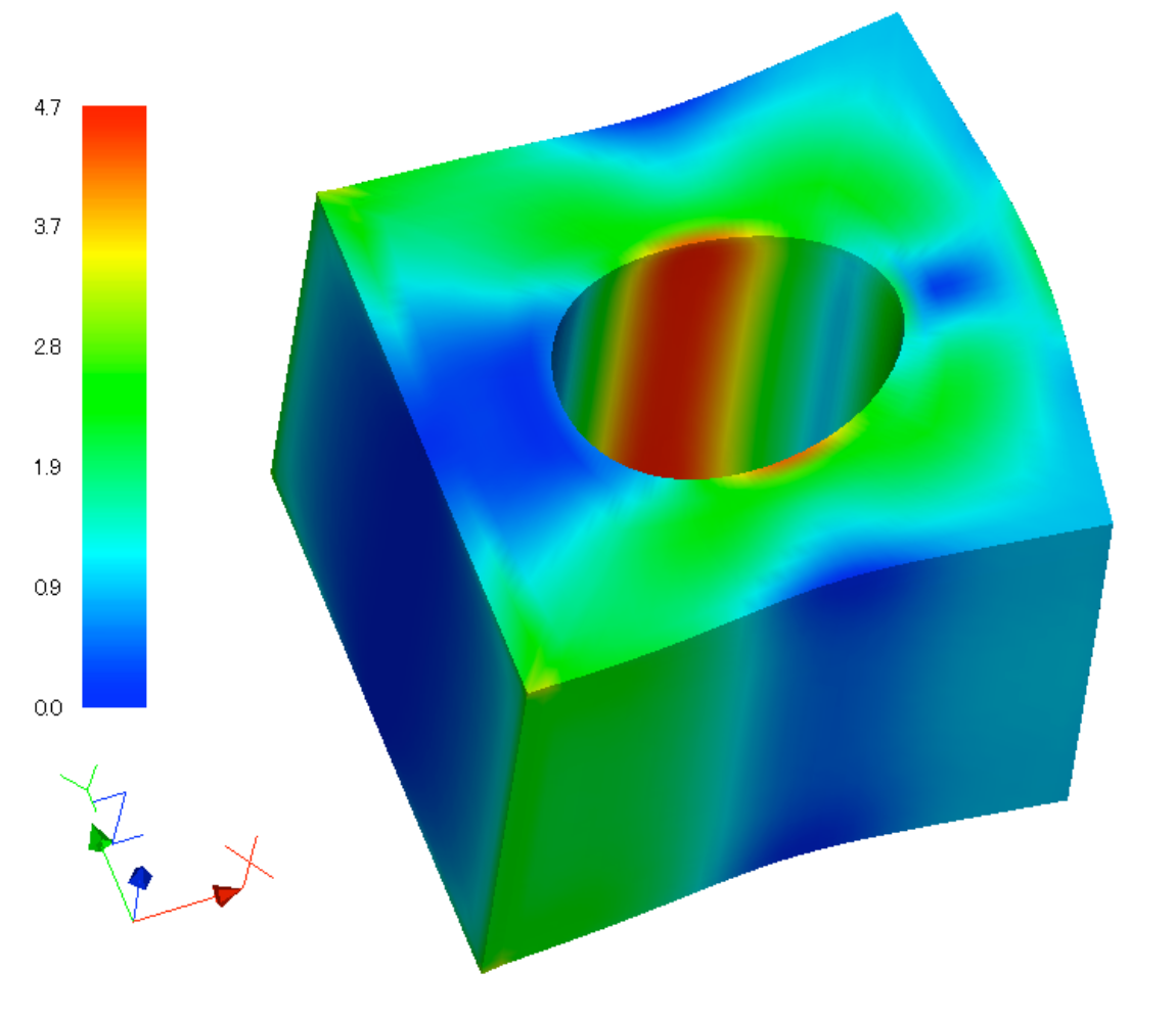
EX02	361	Block with hole	37,386	112,158
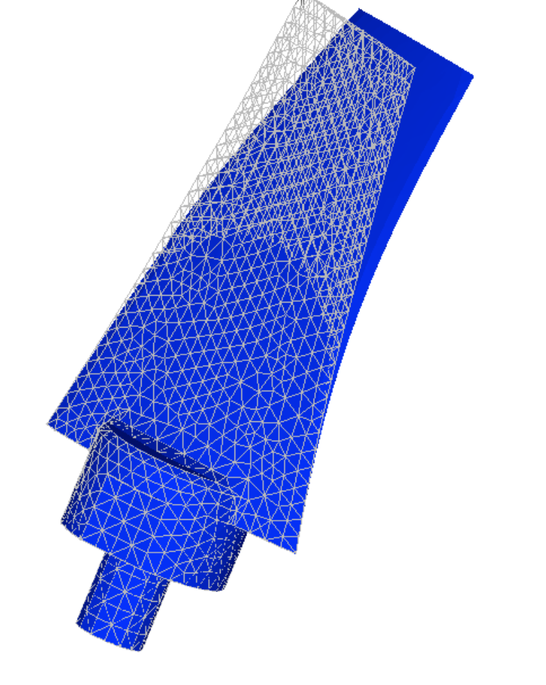
EX03	342	Turbine blade	10,095	30,285
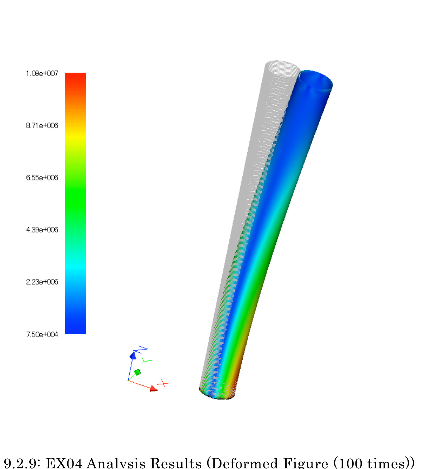
EX04	741	Cylindrical shell	10,100	60,600
EX05A	731	Wine glass (coarse)	7,240	43,440
EX05B	731	Wine glass (midium)	48,803	292,818
EX05C	731	Wine glass (fine)	100,602	603,612

Fig. 9.2.1: Connecting Rod (EX01A)

Fig. 9.2.2: Perforated block (EX02)

Fig. 9.2.3: Turbine blade (EX03, EX06)

Fig. 9.2.4: Cylindrical shell (EX04, EX09)

Fig. 9.2.5: Wine Glass (EX05, EX10A)

Analysis results

Example of analysis results

Examples of the analysis results are shown in Figs. 9.2.6–9.2.9.

Fig. 9.2.6: EX01 analysis results (Mises stress and deformation diagram (10 times))

Fig. 9.2.7: EX02 analysis results (Mises stress and deformation diagram (100 times))

Fig. 9.2.8: EX03 analysis results (deformation diagram (10 times))

Fig. 9.2.9: EX04 analysis results (deformation diagram (100 times))

Verification Results of Analysis Performance with Example EX02

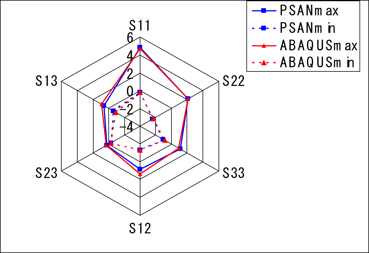
An analysis was performed with the commercial software ABAQUS using a model equivalent to the verification example model EX02 (perforated block). A comparison of the maximum and minimum values of the stress components with the results of FrontISTR is shown in Fig. 9.2.10. It can be seen that the stress components are very close to each other.

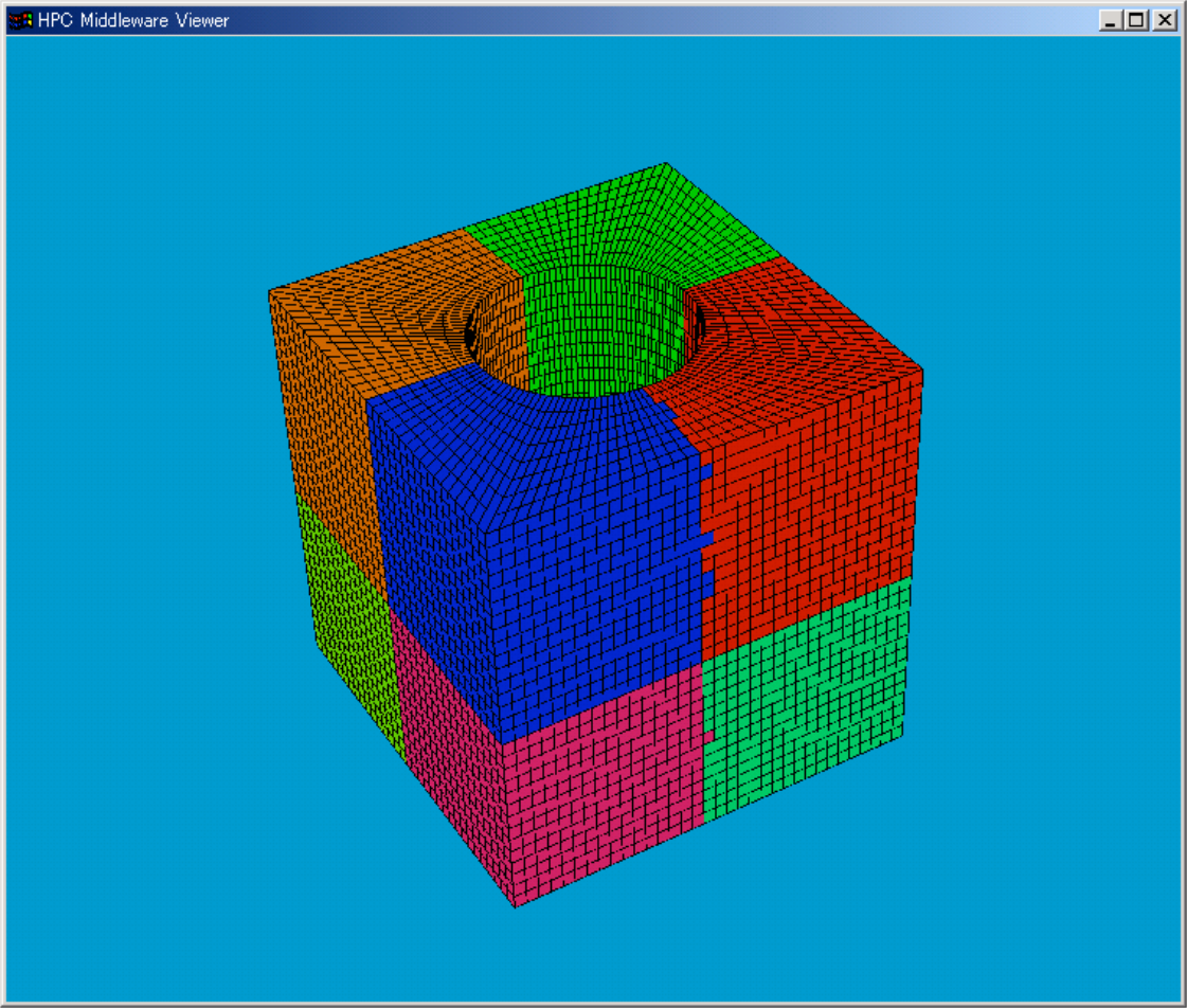
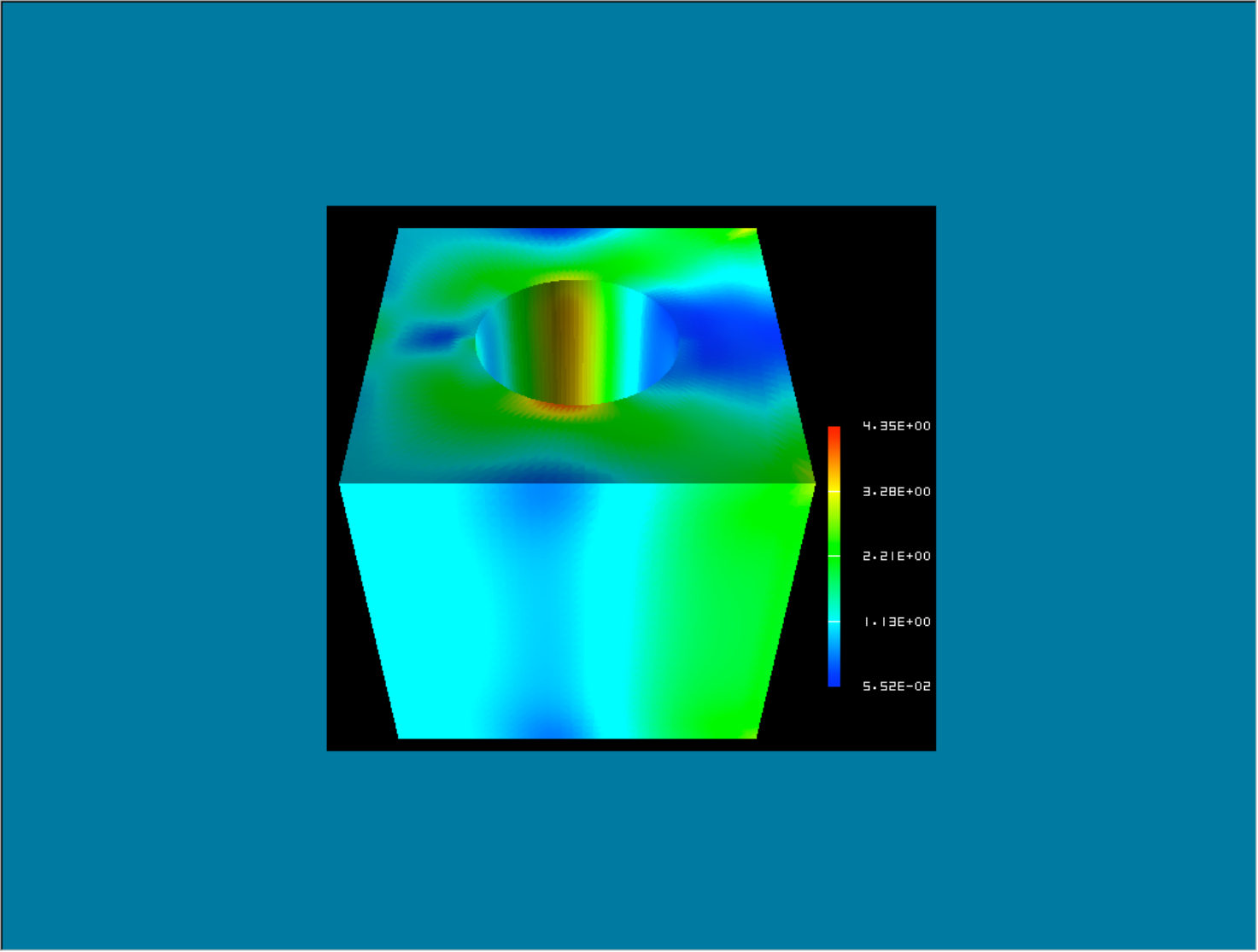
The effect of area division on stress distribution was also analyzed. The division was performed according to the RCB method, i.e., the model was halved in each of the X, Y, and Z axial directions, creating eight areas in total. Fig. 9.2.11 shows the division, while Fig. 9.2.12 shows the stress distribution of the analysis results with a single area and with the area divided into eight areas.

Fig. 9.2.10: Comparison of the stress components of EX02 with the commercial software

Fig. 9.2.11: Result of the division of EX02 in eight areas by the RCB method

Fig. 9.2.12: No difference between the stress distribution of the analysis results with a single area and with the area divided into eight areas

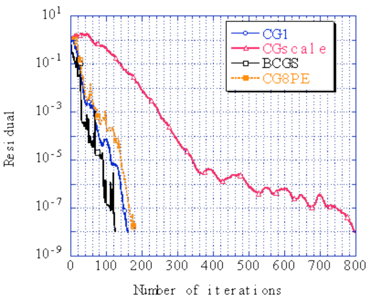
Furthermore, a comparison of the execution time with the settings of the HEC-MW solver used is presented in Table 9.2.2. Fig. 9.2.13 shows the convergence history until the solution was found.

Table 9.2.2: Comparison of execution time with HEC-MW solvers

Solver	Execution Time(s)
CGI	38.79
CGscale	52.75
BCGS	60.79
CG8	6.65

Fig. 9.2.13: Comparison of convergence history with the HEC-MW solver (convergence threshold: \(1.0 \times 10^{-8}\) )

Comparison of calculation time with verification example EX01A

The increase rate of the calculation speed because of area division was verified with the example EX01A (connecting rod.) The test was conducted with a Xeon 2.8 GHz 24 node cluster computer, and the results are shown in Fig. 9.2.14. This figure shows that the calculation speed increases proportionally to the number of areas.

The difference in the calculation time because of the computer environment was also analyzed. The results are presented in Table 9.2.3.

Fig. 9.2.14: Speed-increasing effect because of area division

Table 9.2.3: Comparison of calculation time with different computers (one CPU)

CPU	Frequancy [GHz]	OS	CPU Time [sec]	solver time [sec]
Xeon	2.8	Linux	850	817
Pentium III	0.866	Win2000	2008	1980
Pentium M	0.760	WinXP	1096	1070
Pentium 4	2.0	WinXP	802	785
Pentium 4	2.8	WinXP	738	718
Celeron	0.700	Win2000	2252	2215
Pentium 4	2.4	WinXP	830	804