Infinitesimal Deformation Linear Elasticity Static Analysis

Infinitesimal Deformation Linear Elastic Static Analysis

In this section, the elastic static analysis is formulated on the basis of the infinitesimal deformation theory, which assumes linear elasticity as a stress-strain relationship.

Basic equations

The equilibrium equation, mechanical boundary conditions, and geometric boundary conditions (basic boundary conditions) of solid mechanics are given by the following equations (see Fig. 2.1.1):

$$\begin{equation} \nabla \cdot \sigma + \overline{b} = 0 \quad in \ V \label{eq:2.1.1} \end{equation}$$

$$\begin{equation} \sigma \cdot n = \overline{t} \quad on \ S_t \label{eq:2.1.2} \end{equation}$$

$$\begin{equation} u = \overline{u} \quad on \ S_u \label{eq:2.1.3} \end{equation}$$

where $\sigma$, $\overline{t}$ and $S_t$ denote stress, surface force, and body force, respectively. $S_t$ and $S_u$ represent the geometric and mechanical boundaries, respectively.

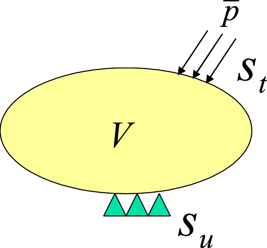
Fig. 2.1.1 Boundary value problem in solid mechanics (infinitesimal deformation problem)

The strain-displacement relation in infinitesimal deformation problems is given by the following equation:

$$\begin{equation} \varepsilon = \nabla_S u \label{eq:2.1.4} \end{equation}$$

Furthermore, the stress-strain relationship (constitutive equation) in linear elastic bodies is given by the following equation:

$$\begin{equation} \sigma = C : \varepsilon \label{eq:2.1.5} \end{equation}$$

where, $C$ is a fourth-order elasticity tensor.

Principle of Virtual Work

The principle of the virtual work related to the infinitesimal deformation linear elasticity problem, which is equivalent to the basic equation Eq.$\eqref{eq:2.1.1}$, Eq.$\eqref{eq:2.1.2}$ and Eq.$\eqref{eq:2.1.3}$, is expressed as:

$$\begin{equation} \int_V \sigma : \delta \varepsilon\, dV = \int_{S_t} \overline{t} \cdot \delta u\, dS + \int_V \overline{b} \cdot \delta u\,dV \label{eq:2.1.6} \end{equation}$$

$$\begin{equation} \delta u = 0 \quad on \ S_u \label{eq:2.1.7} \end{equation}$$

Moreover, considering the constitutive equation Eq.$\eqref{eq:2.1.5}$, Eq.i$\eqref{eq:2.1.6}$, is expressed as follows:

$$\begin{equation} \int_V (C : \varepsilon) : \delta \varepsilon\, dV = \int_{S_t} \overline{t} \cdot \delta u\, dS + \int_V \overline{b} \cdot \delta u\, dV \label{eq:2.1.8} \end{equation}$$

In Eq.$\eqref{eq:2.1.8}$, $\varepsilon$ is the strain tensor and $C$ is the forth-order enasticity tensor. In this case, if the strain tensor $\sigma$ and $\varepsilon$ are represented by vector formats $\hat{\sigma}$ and $\hat{\varepsilon}$, respectively, the consitutive equation Eq.$\eqref{eq:2.1.5}$ is expressed as follows

$$\begin{equation} \hat{\sigma} = D \hat{\varepsilon} \label{eq:2.1.9} \end{equation}$$

where $D$ is an elastic matrix.

Considering that the $\hat{\sigma}$, $\hat{\varepsilon}$ and Eq.$\eqref{eq:2.1.9}$ are expressed in vector format, Eq.$\eqref{eq:2.1.8}$ is expressed as follows:

$$\begin{equation} \int_V \hat{\varepsilon}^T D \delta \hat{\varepsilon}\, dV = \int_{S_t} \delta u^T \overline{t}\, dS + \int_V \delta u^T \overline{b}\, dV \label{eq:2.1.10} \end{equation}$$

Eq.$\eqref{eq:2.1.10}$ and Eq.$\eqref{eq:2.1.7}$ are the principles of the virtual work discretized in this development code.

Formulation

If the principle of virtual work, Eq.$\eqref{eq:2.1.10}$, is discretized for each finite element, the following equation is obtained:

$$\begin{equation} \sum_{e} = \int_{V^e} \hat{\varepsilon}^T D \delta \hat{\varepsilon}\, dV = \sum_{e} \int_{S^e_t} \delta u^T \overline{t}\, dS + \sum_{e} \int_{V^e} \delta u^T \overline{b}\,dV \label{eq:2.1.11} \end{equation}$$

Using the displacement of the nodes that compose each element, the displacement field is interpolated as follows:

$$\begin{equation} u = \sum^m_{i=1} N_i u_i = N U \label{eq:2.1.12} \end{equation}$$

The strain at this moment, using Eq.$\eqref{eq:2.1.4}$, is given as follows:

$$\begin{equation} \hat{\varepsilon} = B U \label{eq:2.1.13} \end{equation}$$

When Eq.$\eqref{eq:2.1.12}$ and Eq.$\eqref{eq:2.1.13}$ are substituted into Eq.$\eqref{eq:2.1.11}$, the following equation is obtained:

$$\begin{equation} \sum_e \delta U^T \left( \int_{V^e} B^T DB\, dV \right) U = \sum_e \delta U^T \cdot \int_{S_t^e} N^T \overline{t}\, dS + \sum_{e} \delta U^T \int_{V^e} N^T \overline{b}\, dV \label{eq:2.1.14} \end{equation}$$

Eq.$\eqref{eq:2.1.14}$ can be summarized as

$$\begin{equation} \delta U^T K U = \delta U^T F \label{eq:2.1.15} \end{equation}$$

In this case, the components of the matrix and vector defined by Eq.$\eqref{eq:2.1.16}$ and Eq.$\eqref{eq:2.1.17}$ can be calculated for each finite and overlapped element:

$$\begin{equation} K = \sum_e \int_{V^e} B^T DB dV \label{eq:2.1.16} \end{equation}$$

$$\begin{equation} F = \sum_e (\int_{S_t^e} N^T \overline{t}\, dS + \int_{V^e} N^T \overline{b}\, dV ) \label{eq:2.1.17} \end{equation}$$

if Eq.$\eqref{eq:2.1.15}$ is true for an arbitary virtual displacement $\delta U$, tha following equation is obtained:

$$\begin{equation} K U = F \label{eq:2.1.18} \end{equation}$$

Meanwhile, the displacement boundary conditioni Eq.$\eqref{eq:2.1.3}$ is expressed as follows:

$$\begin{equation} U = \overline{U} \label{eq:2.1.19} \end{equation}$$

By solving Eq.$\eqref{eq:2.1.18}$ based on the constraint condition Eq.$\eqref{eq:2.1.19}$, it is possible to define the node displacement $U$.