Linear Dynamic Analysis

This analysis uses the data of tutorial/12_dynamic_beam.

Analysis target

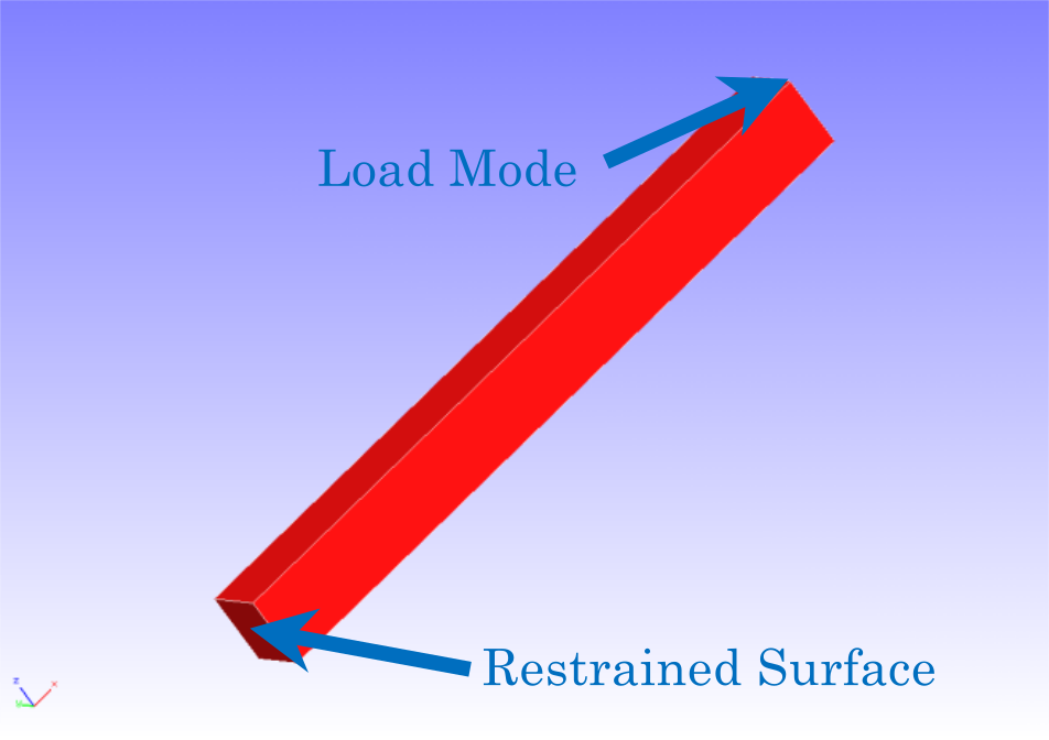
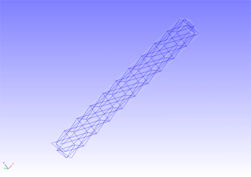
The analysis target is a cantilevered beam, and the geometry is shown in Figure 4.12.1 and the mesh data is shown in Figure 4.12.2.

Item	Description	Notes
Type of analysis	Linear dynamic analysis	!SOLUTION,TYPE=DYNAMIC !DYNAMIC,TYPE=LINEAR
Number of nodes	525
Number of elements	240
Element type	Ten node tetrahedral quadratic element	!ELEMENT,TYPE=342
Material name	M1
Boundary conditions	Restraint,Concentrated force	!CLOAD
Matrix solution	CG/SSOR	!SOLVER,METHOD=CG,PRECOND=1

Shape of the cantilever

Fig. 4.12.1: Shape of the cantilever

Mesh data of the cantilever

Fig. 4.12.2: Mesh data of the cantilever

Analysis contents

A linear dynamic analysis is performed after the displacement of the restraining surface shown in Figure 4.12.1 is restrained and a concentrated load is applied to the load nodes. The analytical control data are shown below.

Analysis control data `beam.cnt`.

#  Control File for FISTR
## Analysis Control
!VERSION
 3
!WRITE,LOG,FREQUENCY=5000
!WRITE,RESULT,FREQUENCY=5000
!SOLUTION, TYPE=DYNAMIC
!DYNAMIC, TYPE=LINEAR
 11 , 1
 0.0, 1.0, 500000, 1.0000e-8
 0.5, 0.25
 1, 1, 0.0, 0.0
 100000, 3121, 500
 1, 1, 1, 1, 1, 1
## Solver Control
### Boundary Conditon
!BOUNDARY, AMP=AMP1
 FIX, 1, 3, 0.0
!CLOAD, AMP=AMP1
 CL1,    3,    -1.0
### Material
# define in mesh file
### Solver Setting
!SOLVER,METHOD=CG,PRECOND=1,ITERLOG=NO,TIMELOG=NO
 10000, 1
 1.0e-06, 1.0, 0.0
!END

Analysis procedure

Execute the FrontISTR execution command fistr1.

$ cd FrontISTR/tutorial/12_dynamic_beam
$ fistr1 -t 4
(Runs in 4 threads.)

Analysis results

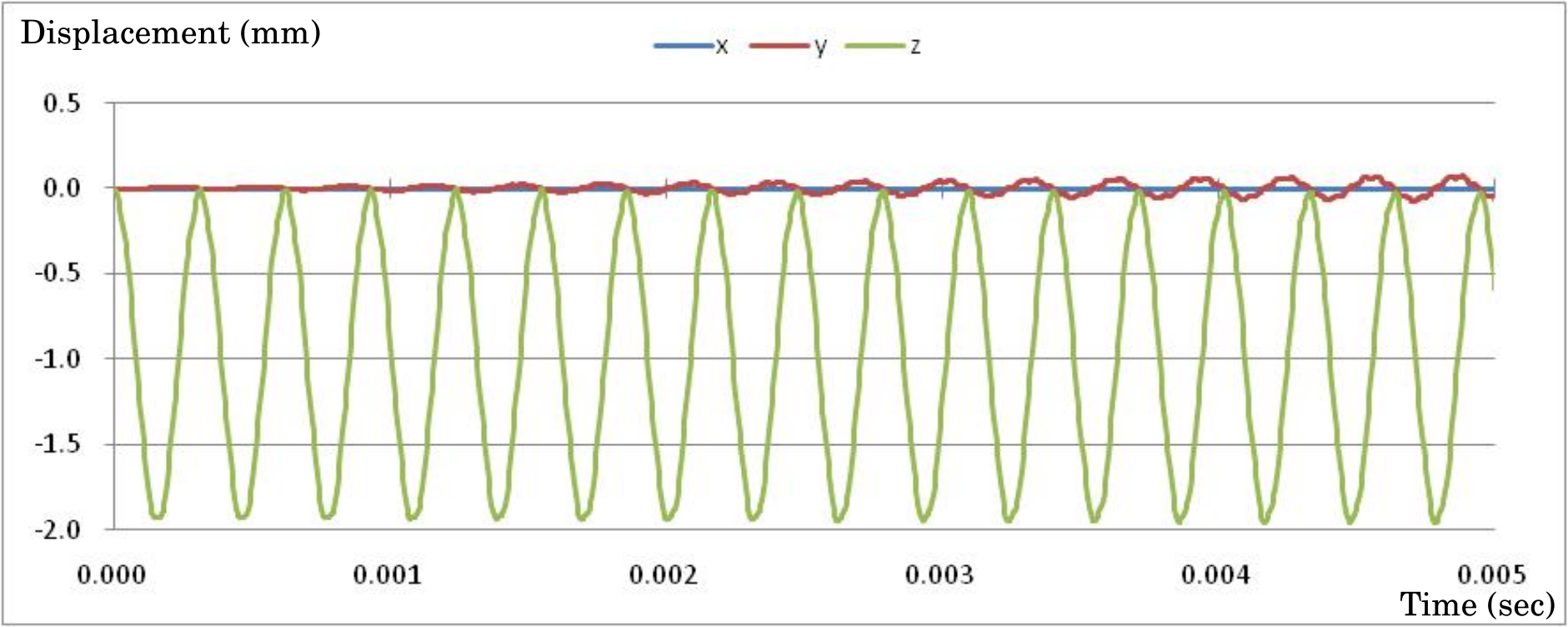
Figure 4.12.3 shows a time series of the displacement of a monitoring node (load node, 3121) specified in the analysis control data, created by Microsoft Excel. A part of the monitoring node displacement output file (dyna_disp_3121.txt) is shown below as numerical data for the analysis results.

Time-series displacement of monitoring nodes

Fig. 4.12.3: Time-series displacement of monitoring nodes

         0  0.0000E+000      3121  0.0000E+000  0.0000E+000  0.0000E+000
       500  5.0000E-006      3121  5.3301E-005 -2.6682E-005 -1.5646E-002
      1000  1.0000E-005      3121  4.0790E-005 -1.0696E-006 -4.4118E-002
      1500  1.5000E-005      3121  9.1017E-005  5.7542E-005 -8.1017E-002
      2000  2.0000E-005      3121  1.8944E-005  5.6499E-005 -1.2358E-001
      2500  2.5000E-005      3121  3.4535E-005  6.1147E-005 -1.7787E-001
      3000  3.0000E-005      3121  3.0248E-005  1.6211E-004 -2.2844E-001
      3500  3.5000E-005      3121  4.2434E-005  1.1706E-004 -2.7330E-001
      4000  4.0000E-005      3121 -2.0130E-005  1.2298E-004 -3.2436E-001
      4500  4.5000E-005      3121  4.1976E-005 -4.2753E-005 -3.8902E-001
      5000  5.0000E-005      3121  5.6526E-005  1.2043E-004 -4.6494E-001
      5500  5.5000E-005      3121  1.9195E-005  8.8901E-006 -5.4673E-001
      6000  6.0000E-005      3121  3.9722E-005 -8.0492E-005 -6.4665E-001
      6500  6.5000E-005      3121  9.0688E-005 -1.9603E-004 -7.5697E-001
      7000  7.0000E-005      3121  3.8175E-005  1.3406E-004 -8.6961E-001
      7500  7.5000E-005      3121 -2.1776E-005  2.9617E-004 -9.6952E-001
      8000  8.0000E-005      3121 -1.6732E-005  2.0223E-004 -1.0672E+000
      8500  8.5000E-005      3121  1.0129E-004  4.9717E-004 -1.1583E+000
      9000  9.0000E-005      3121  4.4797E-005  6.6073E-004 -1.2421E+000
      9500  9.5000E-005      3121 -5.5023E-007  7.2865E-004 -1.3154E+000
     10000  1.0000E-004      3121  4.6793E-005  3.6134E-004 -1.3947E+000

Linear Dynamic Analysis