Linear Static Analysis (Elasticity)
Linear Static Analysis (Elasticity)
For this analysis, the data in tutorial/01_elastic_hinge is used.
Analysis target
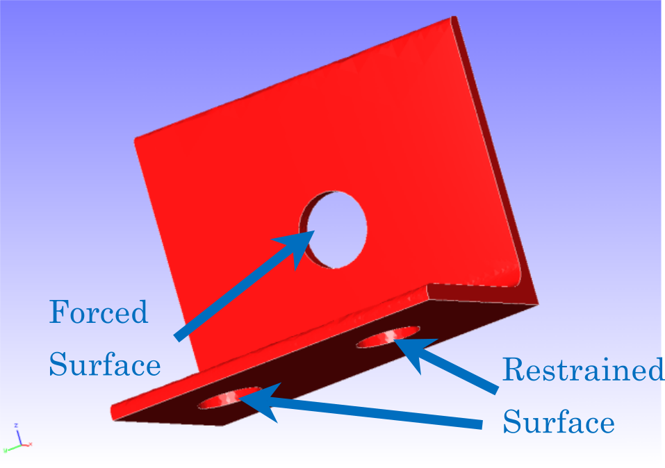
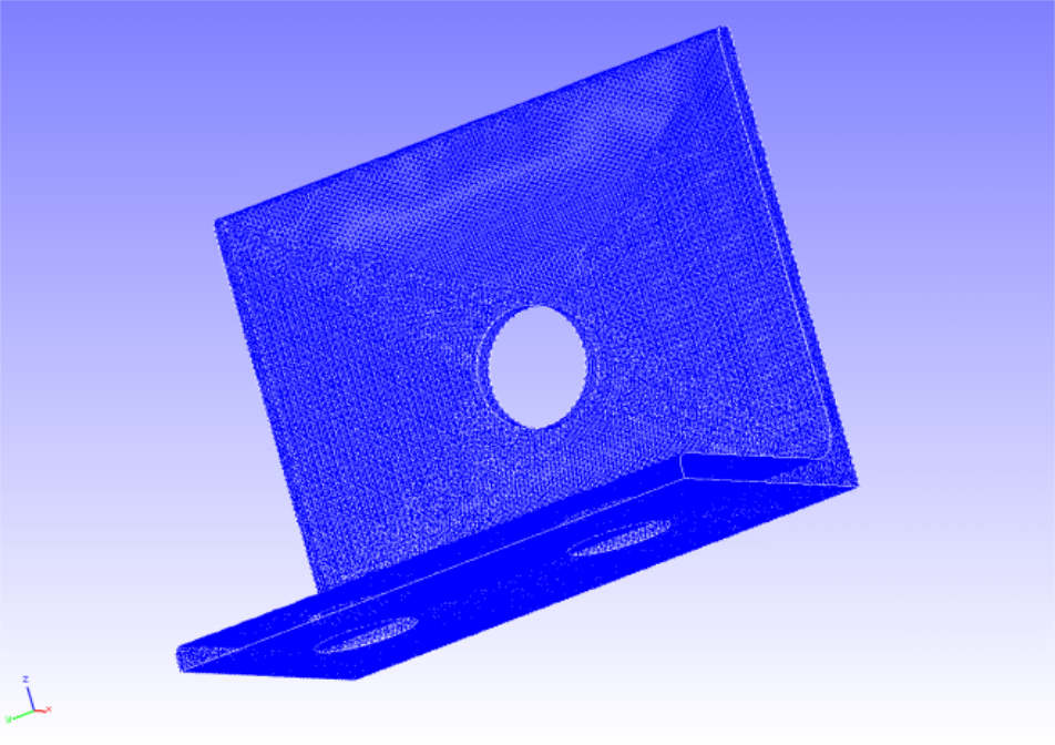
The analysis object is a hinge part, and the geometry is shown in Figure 4.1.1 and the mesh data in Figure 4.1.2.
| Item | Description | Notes | Reference |
|---|---|---|---|
| Type of analysis | Linear static analysis | !SOLUTION,TYPE=STATIC | |
| Number of nodes | 84,056 | ||
| Number of elements | 49,871 | ||
| Element type | 10-node tetrahedron quadratic element | !ELEMENT,TYPE=342 | Element Library |
| Material Name | STEEL | !ELASTIC | Material Data |
| Material property | ELASTIC | ||
| Boudary condition | Restrained, Concentrated force | ||
| Matrix solution | CG/SSOR | !SOLVER,METHOD=CG,PRECOND=1 |
Analysis target
Extract the source code of FrontISTR and go to the directory of this example to see if you can find the files necessary for analysis.
| File name | Type | Role |
|---|---|---|
hecmw_ctrl.dat |
Global control data | Specifies the input and output files for mesh data and analysis control data. |
hinge.cnt |
Analysis control data | Define the type of analysis, displacement boundary conditions, concentrated loads, etc., and also specify control of the solver and visualizer. |
hinge.msh |
Mesh data | Defines a finite element mesh and defines its material and section data |
$ tar xvf FrontISTR.tar.gz
$ cd FrontISTR/tutorial/01_elastic_hinge
$ ls
hecmw_ctrl.dat  hinge.cnt  hinge.msh
A stress analysis is performed to constrain the displacement of the constrained surface shows in Figure 4.1.1 and to apply concentrated loads to the forcing surface.
The overall control data and analytical control data are shown below.
Global control data hecmw_ctrl.dat
#
# for solver
#
!MESH, NAME=fstrMSH, TYPE=HECMW-ENTIRE # Specify a single mesh data
 hinge.msh
!CONTROL, NAME=fstrCNT                 # Specify analysis control data
 hinge.cnt
!RESULT, NAME=fstrRES, IO=OUT          # Specify the result data
 hinge.res
!RESULT, NAME=vis_out, IO=OUT          # Specify visualization data
 hinge_vis
Analysis control data hinge.cnt
#  Control File for FISTR
## Analysis Control
!VERSION                   # Specify the version of the file format
 3
!SOLUTION, TYPE=STATIC     # Specify the type of analysis
!WRITE,RESULT              # Specify the output of the result data
!WRITE,VISUAL              # Specify the output of the visualization data
## Solver Control
### Boundary Conditon
!BOUNDARY
 BND0, 1, 3, 0.000000      # Restrained surface 1
!BOUNDARY
 BND1, 1, 3, 0.000000      # Restrained surface 2
!CLOAD
 CL0, 1, 0.01000           # Specify a forced surface
### Material
!MATERIAL, NAME=STEEL      # Specify material properties
!ELASTIC                   # Definition of elastic substances
 210000.0, 0.3
!DENSITY                   # Definition of mass density
 7.85e-6
### Solver Setting
!SOLVER,METHOD=CG,PRECOND=1,ITERLOG=YES,TIMELOG=YES  # Solver control
 10000, 1
 1.0e-08, 1.0, 0.0
## Post Control
!VISUAL,metod=PSR           # Specify the visualization method
!surface_num=1              # Number of surfaces in one surface rendering
!surface 1                  # Specify the contents of the surface
!output_type=VTK            # Specify the type of the visualization file
!END                        # Indicates the end of the analysis control data
Mesh data
(Some only)
!HEADER
 HECMW_Msh File generated by REVOCAP
!NODE
       1,    -1.22042,     2.23355,     1.65220
       2,    -1.27050,    -3.10529,     1.59209
...
!ELEMENT, TYPE=342
       1,    1157,    3549,    3321,    3739,   12629,   12627,   12626,   12628,   12631,   12630
       2,    8207,    3321,    3549,    3739,   12629,   12633,   12632,   12634,   12630,   12631
...
!MATERIAL, NAME=STEEL, ITEM=2
!ITEM=1, SUBITEM=2
210000.0, 0.3
!ITEM=2, SUBITEM=1
7.85e-6
!SECTION, TYPE=SOLID, EGRP=Solid0, MATERIAL=STEEL
!EGROUP, EGRP=Solid0
1
2
...
!END
Analysis procedure
Execute the FrontISTR command fistr1.
$ fistr1 -t 4
(Runs in 4 threads.)
##################################################################
#                         FrontISTR
#
##################################################################
---
version:    5.1.0
git_hash:   acab000c8c633b7b9d596424769e14363f720841
build:
  date:     2020-10-05T07:39:55Z
  MPI:      enabled
  OpenMP:   enabled
  option:   "-p --with-tools --with-refiner --with-metis --with-mumps --with-lapack --with-ml --with-mkl "
  HECMW_METIS_VER: 5
execute:
  date:       2020-10-07T10:01:16+0900
  processes:  1
  threads:    4
  cores:      4
  host:
    0: flow-p06
---
...
 Step control not defined! Using default step=1
 fstr_setup: OK
 Start visualize PSF 1 at timestep 0

 loading step=    1
 sub_step= 1,   current_time=  0.0000E+00, time_inc=  0.1000E+01
 loading_factor=    0.0000000   1.0000000
### 3x3 BLOCK CG, SSOR, 1
      1    1.903375E+00
      2    1.974378E+00
      3    2.534627E+00
...
...
   2967    1.080216E-08
   2968    1.004317E-08
   2969    9.375729E-09
### Relative residual = 9.39429E-09

### summary of linear solver
      2969 iterations      9.394286E-09
    set-up time      :     1.953022E-01
    solver time      :     5.704201E+01
    solver/comm time :     5.145826E-01
    solver/matvec    :     2.306329E+01
    solver/precond   :     2.632665E+01
    solver/1 iter    :     1.921253E-02
    work ratio (%)   :     9.909789E+01

 Start visualize PSF 1 at timestep 1
### FSTR_SOLVE_NLGEOM FINISHED!

 ====================================
    TOTAL TIME (sec) :     59.99
           pre (sec) :      0.71
         solve (sec) :     59.29
 ====================================
 FrontISTR Completed !!
The analysis is completed when FrontISTR Completed !! is displayed, the analysis is done.
Analysis results
Once the analysis is complete, several new files will be created.
$ ls
0.log       hecmw_ctrl.dat  hinge.res.0.0            hinge_vis_psf.0001
FSTR.dbg.0  hecmw_vis.ini   hinge.res.0.1            hinge_vis_psf.0001.pvtu
FSTR.msg    hinge.cnt       hinge_vis_psf.0000
FSTR.sta    hinge.msh       hinge_vis_psf.0000.pvtu
The *.res.* is the result data of FrontISTR, which can be displayed by REVOCAP_PrePost and so on.
The *_vis_* is called visualization data, and can be displayed by general-purpose visualization software. In this example, the data is output in VTK format, so it can be displayed using ParaView and other visualization software.
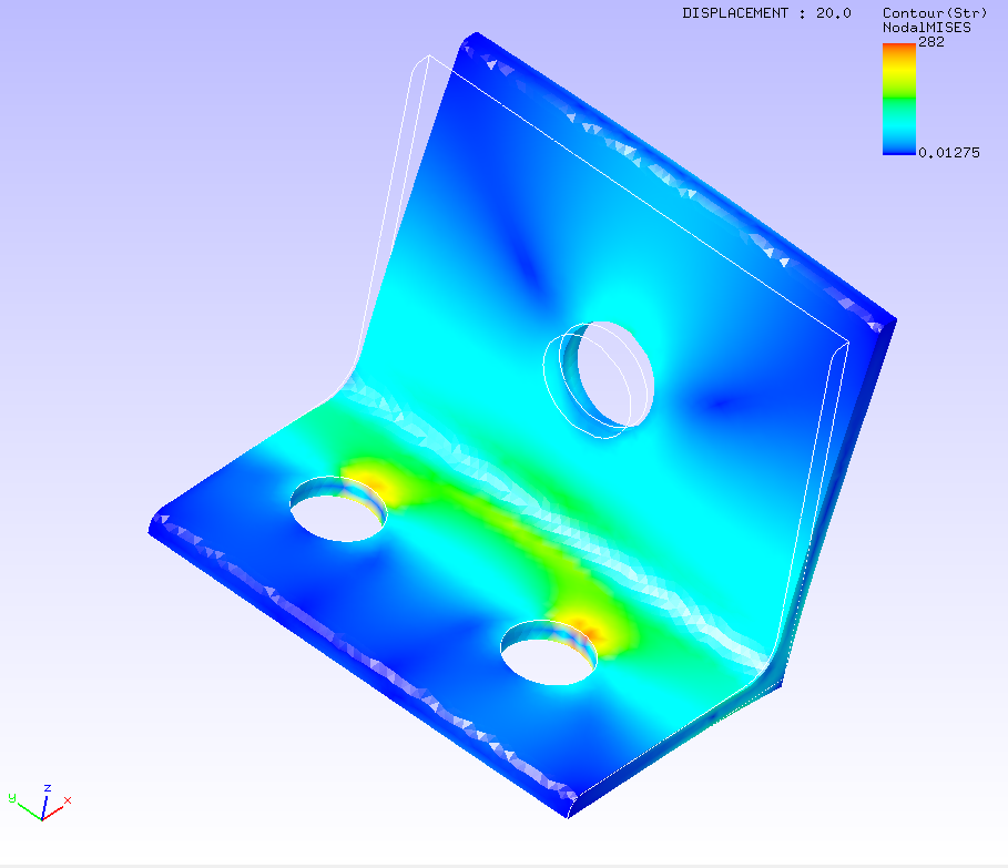
A contour plot for the Mises stresses is created by REVOCAP_PrePost and shown in Figure 4.1.3. A portion of the analysis results log file is also shown below as numerical data for the analysis results.
Log file 0.log
 fstr_setup: OK
#### Result step=     0
 ##### Local Summary @Node    :Max/IdMax/Min/IdMin####
 //U1    0.0000E+00         1  0.0000E+00         1
 //U2    0.0000E+00         1  0.0000E+00         1
 //U3    0.0000E+00         1  0.0000E+00         1
 //E11   0.0000E+00         1  0.0000E+00         1
 //E22   0.0000E+00         1  0.0000E+00         1
 //E33   0.0000E+00         1  0.0000E+00         1
 //E12   0.0000E+00         1  0.0000E+00         1
 //E23   0.0000E+00         1  0.0000E+00         1
 //E31   0.0000E+00         1  0.0000E+00         1
 //S11   0.0000E+00         1  0.0000E+00         1
 //S22   0.0000E+00         1  0.0000E+00         1
 //S33   0.0000E+00         1  0.0000E+00         1
 //S12   0.0000E+00         1  0.0000E+00         1
 //S23   0.0000E+00         1  0.0000E+00         1
 //S31   0.0000E+00         1  0.0000E+00         1
 //SMS   0.0000E+00         1  0.0000E+00         1
 ##### Local Summary @Element :Max/IdMax/Min/IdMin####
 //E11   0.0000E+00         1  0.0000E+00         1
 //E22   0.0000E+00         1  0.0000E+00         1
 //E33   0.0000E+00         1  0.0000E+00         1
 //E12   0.0000E+00         1  0.0000E+00         1
 //E23   0.0000E+00         1  0.0000E+00         1
 //E31   0.0000E+00         1  0.0000E+00         1
 //S11   0.0000E+00         1  0.0000E+00         1
 //S22   0.0000E+00         1  0.0000E+00         1
 //S33   0.0000E+00         1  0.0000E+00         1
 //S12   0.0000E+00         1  0.0000E+00         1
 //S23   0.0000E+00         1  0.0000E+00         1
 //S31   0.0000E+00         1  0.0000E+00         1
 //SMS   0.0000E+00         1  0.0000E+00         1
 ##### Global Summary @Node    :Max/IdMax/Min/IdMin####
 //U1    0.0000E+00         1  0.0000E+00         1
 //U2    0.0000E+00         1  0.0000E+00         1
 //U3    0.0000E+00         1  0.0000E+00         1
 //E11   0.0000E+00         1  0.0000E+00         1
 //E22   0.0000E+00         1  0.0000E+00         1
 //E33   0.0000E+00         1  0.0000E+00         1
 //E12   0.0000E+00         1  0.0000E+00         1
 //E23   0.0000E+00         1  0.0000E+00         1
 //E31   0.0000E+00         1  0.0000E+00         1
 //S11   0.0000E+00         1  0.0000E+00         1
 //S22   0.0000E+00         1  0.0000E+00         1
 //S33   0.0000E+00         1  0.0000E+00         1
 //S12   0.0000E+00         1  0.0000E+00         1
 //S23   0.0000E+00         1  0.0000E+00         1
 //S31   0.0000E+00         1  0.0000E+00         1
 //SMS   0.0000E+00         1  0.0000E+00         1
 ##### Global Summary @Element :Max/IdMax/Min/IdMin####
 //E11   0.0000E+00         1  0.0000E+00         1
 //E22   0.0000E+00         1  0.0000E+00         1
 //E33   0.0000E+00         1  0.0000E+00         1
 //E12   0.0000E+00         1  0.0000E+00         1
 //E23   0.0000E+00         1  0.0000E+00         1
 //E31   0.0000E+00         1  0.0000E+00         1
 //S11   0.0000E+00         1  0.0000E+00         1
 //S22   0.0000E+00         1  0.0000E+00         1
 //S33   0.0000E+00         1  0.0000E+00         1
 //S12   0.0000E+00         1  0.0000E+00         1
 //S23   0.0000E+00         1  0.0000E+00         1
 //S31   0.0000E+00         1  0.0000E+00         1
 //SMS   0.0000E+00         1  0.0000E+00         1
#### Result step=     1
 ##### Local Summary @Node    :Max/IdMax/Min/IdMin####
 //U1    3.9115E-02     82452 -7.1083E-04     65233
 //U2    7.4504E-05       354 -5.8813E-04       696
 //U3    5.9493E-04        84 -5.8751E-03     61080
 //E11   1.3777E-03       130 -1.3653E-03     77625
 //E22   4.9199E-04        61 -5.4370E-04       102
 //E33   6.8634E-04     51036 -6.1176E-04     30070
 //E12   7.1556E-04     27808 -6.8093E-04     27863
 //E23   5.3666E-04        56 -5.4347E-04        82
 //E31   7.2396E-04     36168 -9.6621E-04       130
 //S11   3.8626E+02       130 -3.6387E+02     28580
 //S22   1.6628E+02       130 -1.5743E+02     28580
 //S33   1.6502E+02     30033 -1.5643E+02     28580
 //S12   5.7795E+01     27808 -5.4998E+01     27863
 //S23   4.3345E+01        56 -4.3896E+01        82
 //S31   5.8474E+01     36168 -7.8040E+01       130
 //SMS   2.8195E+02     77625  1.2755E-02     75112
 ##### Local Summary @Element :Max/IdMax/Min/IdMin####
 //E11   1.0731E-03     10485 -1.2123E-03     41779
 //E22   3.9143E-04     33536 -4.1389E-04     22892
 //E33   5.9415E-04     44563 -5.0497E-04     47965
 //E12   5.3264E-04      9163 -5.0405E-04      9161
 //E23   3.9226E-04     33024 -4.1464E-04     23465
 //E31   5.7633E-04     43142 -4.8019E-04      9571
 //S11   2.7231E+02      9180 -2.9763E+02     41779
 //S22   1.0792E+02      9180 -1.0656E+02     41779
 //S33   1.3921E+02     44569 -1.1431E+02     47974
 //S12   4.3021E+01      9163 -4.0712E+01      9161
 //S23   3.1683E+01     33024 -3.3490E+01     23465
 //S31   4.6550E+01     43142 -3.8785E+01      9571
 //SMS   2.4057E+02     41779  3.1383E-02     38687
 ##### Global Summary @Node    :Max/IdMax/Min/IdMin####
 //U1    3.9115E-02     82452 -7.1083E-04     65233
 //U2    7.4504E-05       354 -5.8813E-04       696
 //U3    5.9493E-04        84 -5.8751E-03     61080
 //E11   1.3777E-03       130 -1.3653E-03     77625
 //E22   4.9199E-04        61 -5.4370E-04       102
 //E33   6.8634E-04     51036 -6.1176E-04     30070
 //E12   7.1556E-04     27808 -6.8093E-04     27863
 //E23   5.3666E-04        56 -5.4347E-04        82
 //E31   7.2396E-04     36168 -9.6621E-04       130
 //S11   3.8626E+02       130 -3.6387E+02     28580
 //S22   1.6628E+02       130 -1.5743E+02     28580
 //S33   1.6502E+02     30033 -1.5643E+02     28580
 //S12   5.7795E+01     27808 -5.4998E+01     27863
 //S23   4.3345E+01        56 -4.3896E+01        82
 //S31   5.8474E+01     36168 -7.8040E+01       130
 //SMS   2.8195E+02     77625  1.2755E-02     75112
 ##### Global Summary @Element :Max/IdMax/Min/IdMin####
 //E11   1.0731E-03     10485 -1.2123E-03     41779
 //E22   3.9143E-04     33536 -4.1389E-04     22892
 //E33   5.9415E-04     44563 -5.0497E-04     47965
 //E12   5.3264E-04      9163 -5.0405E-04      9161
 //E23   3.9226E-04     33024 -4.1464E-04     23465
 //E31   5.7633E-04     43142 -4.8019E-04      9571
 //S11   2.7231E+02      9180 -2.9763E+02     41779
 //S22   1.0792E+02      9180 -1.0656E+02     41779
 //S33   1.3921E+02     44569 -1.1431E+02     47974
 //S12   4.3021E+01      9163 -4.0712E+01      9161
 //S23   3.1683E+01     33024 -3.3490E+01     23465
 //S31   4.6550E+01     43142 -3.8785E+01      9571
 //SMS   2.4057E+02     41779  3.1383E-02     38687